Non-Maxwellian Velocity Statistics in Supercooled Liquids and Their Possible Relation to Super-Arrhenius Viscosity
Pith reviewed 2026-07-02 17:18 UTC · model grok-4.3
The pith
Supercooled liquids develop persistent non-Maxwellian velocity distributions because long-lived metastable states support finite-width temperature fluctuations.
A machine-rendered reading of the paper's core claim, the machinery that carries it, and where it could break.
Core claim
Long-lived metastable states in supercooled liquids allow a distribution of temperatures whose dimensionless width A_bar produces non-Maxwellian velocity statistics with excess kurtosis κ ≃ 3 A_bar². Custom stochastic thermostats that do not enforce Maxwellian velocities generate long-lived states with 0 < κ ≲ 0.3 whose crystallization is impeded as κ rises. The nearly constant A_bar ≈ 0.08 extracted from viscosity collapse across 45 materials and from specific-heat data is consistent with the kurtosis measured in the simulations, thereby connecting non-Maxwellian velocities to super-Arrhenius relaxation.
What carries the argument
Stochastic thermostats that maintain stationary states without imposing Maxwellian velocity distributions, together with the relation κ ≃ 3 A_bar² that converts the dimensionless temperature-fluctuation width A_bar into observed kurtosis.
If this is right
- Crystallization is strongly impeded as excess kurtosis increases.
- A single nearly constant temperature-fluctuation width A_bar collapses viscosity data for 45 different glass formers.
- The same width reproduces the kurtosis seen in the non-equilibrium simulations.
- Non-Maxwellian velocity statistics therefore connect slow relaxation, transport coefficients, and thermodynamic measurements.
Where Pith is reading between the lines
- The same mechanism could apply to other long-lived metastable systems whose intensive variables fluctuate, such as certain protein conformations or jammed granular packings.
- Standard molecular-dynamics thermostats that enforce Maxwellian velocities may systematically miss dynamical features present in real supercooled liquids.
- Direct experimental probes of velocity histograms in colloidal or molecular glass formers near the glass transition would test the predicted excess kurtosis.
Load-bearing premise
Long-lived metastable states can sustain a finite-width distribution of an intensive variable such as temperature.
What would settle it
A simulation or measurement that finds strictly Maxwellian velocity distributions (κ = 0) in a deeply supercooled liquid whose relaxation time follows strong super-Arrhenius growth would falsify the proposed link.
Figures


read the original abstract
For particles of fixed mass, classical equilibrium statistical mechanics dictates a Maxwellian velocity distribution determined solely by the temperature, regardless of the interactions, density, or structure. Supercooled glass forming liquids realize long lived metastable states that evade equilibrium crystallization and may thus violate assumptions underlying Maxwellian statistics. We numerically demonstrate that supercooled liquids can exhibit persistent non-Maxwellian velocity distributions with deviations connected to their exceptionally slow super-Arrhenius relaxation. Our work is motivated by a general result establishing that long lived metastable states may exhibit finite width distributions of intensive variables. A distribution of temperatures implies non-Maxwellian velocity statistics. We test this prediction by introducing stochastic thermostats that generate stationary states while, unlike conventional thermostats, not imposing Maxwellian velocity distributions. Simulations with these thermostats yield long lived states that have, by comparison to Maxwellian velocity distributions, an excess kurtosis $0<\kappa\lesssim0.3$. Crystallization is strongly impeded with increasing $\kappa$. In a minimal description, temperature fluctuations are characterized by a dimensionless width $\overline{A}$ with $\kappa\simeq3\overline{A}^{2}$. The nearly constant $\overline{A}$ (of an average value $0.08$ and standard deviation $0.03$) found in viscosity data collapse across $45$ glass formers and in specific heat signatures is consistent with kurtosis found in our simulations. Long time non-Maxwellian velocity statistics may thus link slow relaxation, transport, and thermodynamic measurements. Independent of the tested theory, the stochastic thermostats that we introduce offer a molecular dynamics route to non-Maxwellian velocity statistics.
Editorial analysis
A structured set of objections, weighed in public.
Referee Report
Summary. The manuscript claims that supercooled glass-forming liquids can exhibit persistent non-Maxwellian velocity distributions arising from finite-width temperature fluctuations in long-lived metastable states. This is tested using newly introduced stochastic thermostats that allow non-Maxwellian stationary states, leading to excess kurtosis (0 < κ ≲ 0.3) that impedes crystallization. A minimal model relates kurtosis to a dimensionless temperature fluctuation width A_bar via κ ≃ 3 A_bar², with A_bar ≈ 0.08 extracted from viscosity data collapse over 45 systems and shown consistent with simulation results and specific-heat signatures.
Significance. If the proposed link between non-Maxwellian statistics, temperature fluctuations, and super-Arrhenius relaxation holds, the work would establish a novel connection between velocity distributions, slow dynamics, and thermodynamics in supercooled liquids, while also providing a new molecular dynamics approach to generating non-equilibrium velocity statistics. The introduction of the stochastic thermostats is a potentially useful methodological contribution independent of the theory.
major comments (2)
- [Abstract] Abstract: the quantitative consistency between the fitted A_bar (average value 0.08) from viscosity data collapse across 45 glass formers and the simulated kurtosis relies on the relation κ ≃ 3 A_bar²; since A_bar is determined from the viscosity data to which it is then compared for consistency, this introduces a potential circularity that requires an independent test or a priori prediction of the fluctuation width.
- [Simulations with stochastic thermostats] Simulations section: the central numerical results on excess kurtosis (0 < κ ≲ 0.3) and impeded crystallization are described only at abstract level; without full methods, error analysis on the data-collapse procedure for A_bar, or direct measurement of local temperature fluctuations (or explicit mixture-of-Maxwellians decomposition of the velocity pdf), the link between observed κ and the proposed temperature distribution cannot be assessed.
minor comments (2)
- [Notation] The overbar notation on A_bar should be defined explicitly on first use and used consistently.
- [Introduction] The motivating general result on finite-width distributions of intensive variables in long-lived metastable states would benefit from an explicit citation or brief derivation in the introduction.
Simulated Author's Rebuttal
We thank the referee for the careful reading and constructive comments on our manuscript. We respond point-by-point to the major comments below.
read point-by-point responses
-
Referee: [Abstract] Abstract: the quantitative consistency between the fitted A_bar (average value 0.08) from viscosity data collapse across 45 glass formers and the simulated kurtosis relies on the relation κ ≃ 3 A_bar²; since A_bar is determined from the viscosity data to which it is then compared for consistency, this introduces a potential circularity that requires an independent test or a priori prediction of the fluctuation width.
Authors: We thank the referee for highlighting this point. The value of Ā ≈ 0.08 is extracted exclusively from the viscosity data collapse across the 45 glass formers, which constitutes an independent experimental dataset unrelated to the simulations. The relation κ ≃ 3 Ā^{2} follows directly from the minimal theoretical model of temperature fluctuations (a mixture of Maxwellians). The stochastic-thermostat simulations then provide an independent numerical test by measuring κ directly. The manuscript already cites consistency with specific-heat signatures as a further independent route to Ā. We will revise the abstract and discussion to explicitly emphasize the independence of these datasets and the a priori nature of the specific-heat estimate. revision: partial
-
Referee: [Simulations with stochastic thermostats] Simulations section: the central numerical results on excess kurtosis (0 < κ ≲ 0.3) and impeded crystallization are described only at abstract level; without full methods, error analysis on the data-collapse procedure for A_bar, or direct measurement of local temperature fluctuations (or explicit mixture-of-Maxwellians decomposition of the velocity pdf), the link between observed κ and the proposed temperature distribution cannot be assessed.
Authors: We agree that additional detail is required. In the revised manuscript we will expand the Simulations section with complete implementation details of the stochastic thermostats (algorithms, parameters, and validation). We will include error analysis for the viscosity data-collapse procedure used to obtain Ā. We will also add direct measurements of local temperature fluctuations from the simulations together with an explicit decomposition of the velocity PDF into a mixture of Maxwellians, thereby strengthening the quantitative link between the observed kurtosis and the underlying temperature distribution. revision: yes
Circularity Check
No significant circularity; independent simulations and external data collapse
full rationale
The paper's core numerical result (excess kurtosis 0 < κ ≲ 0.3 in simulations using new stochastic thermostats) is generated independently of the viscosity data. The minimal-model relation κ ≃ 3 A_bar² is used only for a post-hoc consistency check between an A_bar value fitted to separate viscosity collapse across 45 systems and the independently measured simulation kurtosis. No equation reduces the simulation output to the fitted A_bar by construction, and the motivating general result on intensive-variable distributions is not invoked to derive the simulation outcomes. The derivation chain therefore remains self-contained against external benchmarks.
Axiom & Free-Parameter Ledger
free parameters (1)
- A_bar =
0.08
axioms (1)
- domain assumption Long lived metastable states may exhibit finite width distributions of intensive variables
invented entities (1)
-
Temperature distribution (finite width) in supercooled metastable states
no independent evidence
Reference graph
Works this paper leans on
-
[1]
and focus on temperature fluctuations. As repeatedly emphasized above, in all classical equilibrium systems the velocities follow a Maxwellian distribution which is set solely by the temperature and no other equilibrium 10 state variables. This implies that the probability dis- tribution for Cartesian velocity components of a nearly stationary system at n...
-
[2]
sufficient time
OnceP(β|β ′) is known, we can determine numerous quantities for which the temperature is the prominent governing state variable of the supercooled fluid, includ- ing the viscosity as a function of temperature. C. Gamma-Distributed Effective Temperature A fundamental result of equilibrium statistical me- chanics is that the maximization of the entropy subj...
2020
-
[3]
Stationary reduced probability densities The central result of Ref. [4], complementing the framework [5–7, 50, 51, 91], that led to the prediction of non-Maxwellian velocity distributions links the reduced few body (n=O(1)) probability densities of macro- scopic (N≫1) metastable systems to their thermal equilibrium counterparts. Under ensemble equivalence...
-
[4]
(A1) appliesonlyto sta- tionaryρ stationary,n
The linear map of Eq. (A1) appliesonlyto sta- tionaryρ stationary,n. Strictly speaking, it cannot link equilibrium densities to arbitrary time evolv- ing probability densities
-
[5]
|β ′, µ′,
For a bona fide equilibrium system, P(β, µ, . . .|β ′, µ′, . . .) =δ(β ′ −β)δ(µ ′ −µ)· · ·, recovering the standard result
-
[6]
(A1) should also apply to the putative ideal glass (conjectured to be permanently quiescent [3, 92]) whenever ensemble equivalence holds
Eq. (A1) should also apply to the putative ideal glass (conjectured to be permanently quiescent [3, 92]) whenever ensemble equivalence holds. In general, although the system may have a fixed par- ticle number or energy, whenever the reduced few body probability density is stationary the system effectively lies in the convex hull of equilibrium states [4] ...
-
[7]
The ratio of microscopic to crystallization timescales, 10−10 ≳τ micro/τxtal ≳10 −17,(A3) ensures that corrections to Eq
Near stationarity of the supercooled liquid In the metastable supercooled liquid atT > T g, local few body observables are nearly (but not per- fectly) stationary, since crystallization occurs after a fi- nite timeτ xtal. The ratio of microscopic to crystallization timescales, 10−10 ≳τ micro/τxtal ≳10 −17,(A3) ensures that corrections to Eq. (A1) are exce...
-
[8]
Let{ϕ i}N i=1 denote compact local fields (e.g
An origin of finite width ofP(T|T ′) We now outline a mechanism [50] by which the distri- butionP(T|T ′) acquires a finite width. Let{ϕ i}N i=1 denote compact local fields (e.g. local en- ergy or order parameter densities) atNspatial sites, governed by a local HamiltonianH 0[{ϕi}] =P i r 2 ϕ2 i + u 4 ϕ4 i +· · · . During rapid cooling, the external bath c...
-
[9]
smeared out
Viscosity from local observables Setting the observableQin Eq. (A1) to the terminal velocity of a sphere falling through the liquid (Stokes equation), and noting that equilibrium flow occurs only above the liquidus temperatureT l, gives [4–7, 51]: η(T)≃ ηeq.(T + l )R ∞ Tl dT ′P(T|T ′) ,(A13) which with a GaussianP(T|T ′) of width ATyields the erfc collaps...
-
[10]
The two gain termsh(⃗ v ′ 1,2) and two loss termsh(⃗ v 1,2) arise becausef M(⃗ v′ 1)fM(⃗ v′
+h(⃗ v′ 2)−h(⃗ v1)−h(⃗ v2) . The two gain termsh(⃗ v ′ 1,2) and two loss termsh(⃗ v 1,2) arise becausef M(⃗ v′ 1)fM(⃗ v′
-
[11]
=f M(⃗ v1)fM(⃗ v2) by energy conservation. The operatorLis self adjoint and negative semidefinite with respect to the weighted inner product ⟨g, h⟩= R d⃗ v fM(⃗ v)g(⃗ v)h(⃗ v), with kernel spanned by the collision invariants{1, ⃗ v, ⃗ v2}. For Maxwellian particles, it enjoys an eigenfunction expansion in Sonine (associ- ated Laguerre) polynomials [98, 99]...
-
[12]
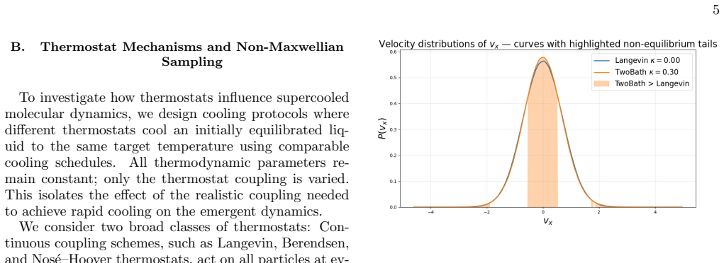
Conventional Thermostats Nos´ e–Hoover The Nos´ e–Hoover thermostat [94] introduces a deter- ministic thermal reservoir through a dynamically evolv- ing friction coefficient that regulates the kinetic tempera- ture. In discrete time, the particle velocities are updated according to ⃗ vi,n+1 =⃗ vi,n + ∆t ⃗Fi,n mi −ζ n ⃗ vi,n ! ,(C1) where the thermostat va...
-
[13]
Collision pairs (i, j) are selected with probability Pcoll = 1−e−ν∆t
Non-Equilibrium Thermostats Heavy-Tailed Lowe–Andersen (HTLA) Thermostat The HTLA thermostat generalizes the conventional stochastic Andersen/Lowe [54] collision scheme by re- placing the Maxwell–Boltzmann post collision velocity sampling with a heavy-tailed kernel. Collision pairs (i, j) are selected with probability Pcoll = 1−e−ν∆t. For each selected pa...
-
[14]
By enforcing this distribution deterministically, it can distort the nat- ural evolution of dynamical observables in non-ergodic or highly heterogeneous states
Drawbacks of Conventional Thermostats The Nos´ e–Hoover thermostat imposes a Maxwell– Boltzmann velocity distribution by design. By enforcing this distribution deterministically, it can distort the nat- ural evolution of dynamical observables in non-ergodic or highly heterogeneous states. The Berendsen thermostat does not generate a true canonical ensembl...
-
[15]
Other metrics of non-Gaussian statistics have been heavily used in earlier studies of supercooled liquids
Non-Gaussian observables The excess (single Cartesian component or other gen- eralized coordinate) velocity kurtosis, is the central quantity analyzed in the current work. Other metrics of non-Gaussian statistics have been heavily used in earlier studies of supercooled liquids. These include, in partic- ular, thedisplacementnon-Gaussian parameter, intro- ...
-
[16]
25 Herein, fast and slow regions coexist and relaxation oc- curs via cooperative rearrangements
Dynamical heterogeneity As noted in the main text, in supercooled liquids, dynamics may become spatially heterogeneous [41–49]. 25 Herein, fast and slow regions coexist and relaxation oc- curs via cooperative rearrangements. Notably, displace- ment distributions develop non-Gaussian tails [3, 103]. The focus of all earlier studies has not been on velociti...
-
[17]
Herein, dynamics are facilitated by neighboring excitations
Kinetically constrained models Kinetically constrained models (KCMs) [22–25], in- cluding the Fredrickson-Andersen (FA) and East mod- els [104–106], capture these features through local mo- bility constraints. Herein, dynamics are facilitated by neighboring excitations. The resulting relaxation is hierarchical and spatially heterogeneous. The struc- tural...
-
[18]
Relation betweenα 2(t)and relaxation The non-Gaussian parameter is related to the variance of the local diffusivityD[107], α2(t)∼ Var(D) ⟨D⟩2 .(D2) As a general rule of thumb trend, increasing non- Gaussianityα 2 appears in tandem with stronger dynam- ical heterogeneity
-
[19]
In a supercooled liquid, nucleation requires collective rearrangements
Connection to the crystallization timeτ xtal The classical nucleation rate is governed by [108] τxtal ∼τ 0 e∆F ∗/T , where ∆F ∗ is the nucleation bar- rier andτ 0 is an attempt timescale. In a supercooled liquid, nucleation requires collective rearrangements. In other words,τ 0 ∼τ α [109] and τxtal ∼τ α e∆F ∗/T .(D3) Sinceα 2(t) peaks at timest∼τ α, its l...
-
[20]
Competing effects of non-Gaussianity Non-Gaussianity has two opposing consequences for crystallization
-
[21]
Largeα 2 signals slow, heterogeneous dynamics⇒ τα ↑⇒τ xtal ↑
-
[22]
superstatistics
Concomitantly, however, similar to the discussion in the main paper (Figs. 12 and 13), fat tails may imply an enhanced tail of fast particles⇒locally enhanced barrier crossing⇒τ xtal ↓. Thusα 2 correlates withτ xtal but does not uniquely de- termine it. E Non-Maxwellian velocity distribu- tions imply correlated constrained dynamics The broadening that we ...
-
[23]
Smallτ Quench ≲10 2 MD step values correspond to rapid quenches that strongly drive the system out of equilibrium and favor glassy arrest
Cooling Rates and Temperature-Time Profiles We cooled the system to time dependent target tem- peratures following an exponential quench protocol, Ttarget(t) =T final + (T0 −T final)e −t/τQuench (G1) whereT 0 is the initial temperature,T final the final target low-temperature state, andτ Quench controls the cooling rate. Smallτ Quench ≲10 2 MD step values...
-
[24]
steady state Verification:F(q, t)as a Probe of Steady State The static structure factorS(⃗ q) quantifies density cor- relations in reciprocal space and is defined as: S(⃗ q) =1 N * NX j=1 NX k=1 e−i⃗ q·(⃗ rj −⃗ rk) + = 1 N * NX j=1 e−i⃗ q·⃗ rj 2+ (G2) Peaks inS(⃗ q) indicate preferred interparticle spacings and provide information about the system’s struc...
-
[25]
Select the final 30%–40% of the trajectory after cooling
-
[26]
Divide this time window intoK= 20 equal seg- ments
-
[27]
ComputeF k(q, t) independently in each segment using only time origins contained within that seg- ment
-
[28]
Stationarity Criterion.We require that the relative spread across these segments satisfy stdk[Fk(q, t)] ⟨Fk(q, t)⟩k ≲3%, t∈α-relaxation window
Compare the resulting curvesF k(q, t). Stationarity Criterion.We require that the relative spread across these segments satisfy stdk[Fk(q, t)] ⟨Fk(q, t)⟩k ≲3%, t∈α-relaxation window. (G3) If the block-averaged curves collapse within approxi- mately 3% throughout the decay region, the system is considered statistically stationary and suitable for reli- abl...
-
[29]
M. D. Ediger, C. A. Angell, and S. R. Nagel, J. Phys. Chem.100, 13200 (1996)
1996
-
[30]
C. A. Angell, Science267, 1924 (1995)
1924
-
[31]
Berthier and G
L. Berthier and G. Biroli, Rev. Mod. Phys.83, 587 (2011)
2011
-
[32]
Nussinov, Ann
Z. Nussinov, Ann. Phys.463, 169634 (2024)
2024
-
[33]
Nussinov, Philos
Z. Nussinov, Philos. Mag.97, 1509 (2017)
2017
-
[34]
N. B. Weingartner, C. Pueblo, F. Nogueira, K. F. Kel- ton, and Z. Nussinov, Front. Mater.3, 50 (2016)
2016
-
[35]
N. B. Weingartner, C. Pueblo, K. F. Kelton, and Z. Nussinov, “Critical assessment of the equilibrium melting-based, energy distribution theory of super- cooled liquids and application to jammed systems,” (2015), arXiv:1512.04565
work page internal anchor Pith review Pith/arXiv arXiv 2015
-
[36]
Vogel, Z
H. Vogel, Z. Phys.22, 645 (1921)
1921
-
[37]
G. S. Fulcher, J. Am. Ceram. Soc.8, 339 (1925)
1925
-
[38]
Tammann and W
G. Tammann and W. Z. Hesse, Anorg. Allgem. Chem. 156, 245 (1926)
1926
-
[40]
P. G. Debenedetti and F. H. Stillinger, Nature410, 259 (2001)
2001
-
[41]
J. Xue, F. S. Nogueira, K. F. Kelton, and Z. Nussinov, Physical Review Research4, 043047 (2022)
2022
-
[42]
J. Zhao, S. L. Simon, and G. B. McKenna, Nat. Com- mun.4, 1783 (2013)
2013
-
[43]
Blodgett, T
M. Blodgett, T. Egami, Z. Nussinov, and K. F. Kelton, Sci. Rep.5, 13837 (2015)
2015
-
[44]
Flenner and G
E. Flenner and G. Szamel, Nat. Commun.6, 7392 (2015)
2015
-
[45]
Illing, S
B. Illing, S. Fritschi, H. Kaiser, C. L. Klix, G. Maret, and P. Keim, Proc. Natl. Acad. Sci. U.S.A.114, 1856 (2017)
2017
-
[46]
Leutheusser, Phys
E. Leutheusser, Phys. Rev. A29, 2765 (1984)
1984
-
[47]
Bengtzelius, W
U. Bengtzelius, W. G¨ otze, and A. Sj¨ olander, J. Phys. C: Solid State Phys.17, 5915 (1984)
1984
-
[48]
G¨ otze,Complex Dynamics of Glass-Forming Liq- uids: A Mode-Coupling Theory(Oxford University Press, 2008)
W. G¨ otze,Complex Dynamics of Glass-Forming Liq- uids: A Mode-Coupling Theory(Oxford University Press, 2008)
2008
-
[49]
L. M. C. Janssen, Front. Phys.6, 97 (2018)
2018
-
[50]
Unified Theory of Activated Relaxation in Liquids over 14 Decades in Time
S. Mirigian and K. S. Schweizer, arXiv:1310.6018 (2013)
work page internal anchor Pith review Pith/arXiv arXiv 2013
-
[51]
R. G. Palmer, D. L. Stein, E. Abrahams, and P. W. Anderson, Phys. Rev. Lett.53, 958 (1984)
1984
- [52]
-
[53]
A. S. Keys, J. P. Garrahan, and D. Chandler, Proc. Natl. Acad. Sci. U.S.A.110, 4482 (2013)
2013
-
[54]
Adam and J
G. Adam and J. H. Gibbs, J. Chem. Phys.43, 139 (1965)
1965
-
[55]
Goldstein, J
M. Goldstein, J. Chem. Phys.51, 3728 (1969). 28
1969
-
[56]
Biroli and J.-P
G. Biroli and J.-P. Bouchaud, inStructural Glasses and Supercooled Liquids: Theory, Experiment, and Applica- tions, edited by P. G. Wolynes and V. Lubchenko (John Wiley & Sons, 2012) pp. 31–113
2012
-
[57]
T. R. Kirkpatrick and P. G. Wolynes, Phys. Rev. B36, 8552 (1987)
1987
-
[58]
T. R. Kirkpatrick, D. Thirumalai, and P. G. Wolynes, Phys. Rev. A40, 1045 (1989)
1989
-
[59]
Lubchenko and P
V. Lubchenko and P. G. Wolynes, Annu. Rev. Phys. Chem.58, 235 (2007)
2007
-
[60]
M´ ezard and G
M. M´ ezard and G. Parisi, J. Chem. Phys.111, 1076 (1999)
1999
-
[61]
Parisi, P
G. Parisi, P. Urbani, and F. Zamponi,Theory of Simple Glasses: Exact Solutions in Infinite Dimensions(Cam- bridge University Press, 2020)
2020
-
[62]
Angelani, G
L. Angelani, G. Parisi, G. Ruocco, and G. Viliani, Phys. Rev. E61, 1681 (2000)
2000
-
[63]
Parisi, Physica A280, 115 (2000)
G. Parisi, Physica A280, 115 (2000)
2000
-
[64]
Charbonneau, J
P. Charbonneau, J. Kurchan, G. Parisi, P. Urbani, and F. Zamponi, Annu. Rev. Condens. Matter Phys.8, 265 (2017)
2017
-
[65]
S. A. Kivelson and G. Tarjus, Nat. Mater.7, 831 (2008)
2008
-
[66]
Kivelson, S
D. Kivelson, S. A. Kivelson, X. Zhao, Z. Nussinov, and G. Tarjus, Physica A219, 27 (1995)
1995
-
[67]
Nussinov, Phys
Z. Nussinov, Phys. Rev. B69, 014208 (2004)
2004
-
[68]
Speck, J
T. Speck, J. Stat. Mech.2019, 084015 (2019)
2019
-
[69]
Sillescu, J
H. Sillescu, J. Non-Cryst. Solids243, 81 (1999)
1999
-
[70]
M. D. Ediger, Annu. Rev. Phys. Chem.51, 99 (2000)
2000
-
[71]
Richert, J
R. Richert, J. Phys.: Condens. Matter14, R703 (2002)
2002
-
[72]
W. Kob, C. Donati, S. J. Plimpton, P. H. Poole, and S. C. Glotzer, Phys. Rev. Lett.79, 2827 (1997)
1997
-
[73]
Donati, J
C. Donati, J. F. Douglas, W. Kob, S. J. Plimpton, P. H. Poole, and S. C. Glotzer, Phys. Rev. Lett.80, 2338 (1998)
1998
-
[74]
Berthier, Physics4, 42 (2011)
L. Berthier, Physics4, 42 (2011)
2011
-
[75]
Zhang, J
P. Zhang, J. J. Maldonis, Z. Liu, J. Schroers, and P. M. Volynes, Nat. Commun.9, 1129 (2018)
2018
-
[76]
Berthier, G
L. Berthier, G. Biroli, J.-P. Bouchaud, L. Cipelletti, and W. van Saarloos,Dynamical Heterogeneities in Glasses, Colloids, and Granular Media(Oxford Uni- versity Press, 2011)
2011
-
[77]
Widmer-Cooper, H
A. Widmer-Cooper, H. Perry, P. Harrowell, and D. R. Reichman, Nat. Phys.4, 711 (2008)
2008
-
[78]
Nussinov, Nucl
Z. Nussinov, Nucl. Phys. B953, 114948 (2020)
2020
-
[79]
Nussinov, N
Z. Nussinov, N. B. Weingartner, and F. S. Nogueira, in Topological Phase Transitions and New Developments, edited by L. Brink, M. Gunn, J. V. Jose, J. M. Koster- litz, and K. K. Phua (World Scientific, 2018) pp. 61–79
2018
-
[80]
S. Nose, J. Chem. Phys.81, 511 (1984)
1984
-
[81]
W. G. Hoover, Phys. Rev. A31, 1695 (1985)
1985
discussion (0)
Sign in with ORCID, Apple, or X to comment. Anyone can read and Pith papers without signing in.