REVIEW 2 major objections 1 minor 55 references
Reviewed by Pith at T0; open to challenge.
T0 means a machine referee read the full paper against a public rubric. The mark states how deep the mechanical check went, never who wrote it. the ladder, T0–T4 →
T0 review · grok-4.3
Growth inserts new neural units into specialized training paths, leaving them with weaker gradient signals than existing units.
2026-06-30 20:51 UTC pith:N7VNTZ53
load-bearing objection Growth isn't the inverse of pruning because new units get starved of gradients when inserted mid-training, but the evidence stays mostly observational. the 2 major comments →
On the Stability of Growth in Structural Plasticity
The pith
A machine-rendered reading of the paper's core claim, the machinery that carries it, and where it could break.
Core claim
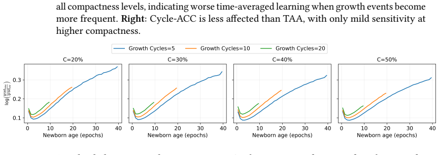
Growth is not the inverse of pruning because newborn units inserted into an already-specialized optimization trajectory participate in the forward computation but receive much weaker gradient signal than incumbent units. This disadvantage is minor in small MLP benchmarks but becomes clear in harder image-classification settings with a convolutional trunk. Interventions on optimizer state, insertion, selection, and trainability can improve integration, yet do not automatically yield better final subnetworks. In continual-learning benchmarks, growth becomes competitive mainly when new units have enough time to integrate.
What carries the argument
The insertion problem, in which new units are forward-active but backward-starved because they enter an already-specialized optimization trajectory.
Load-bearing premise
The observed gradient disadvantage arises specifically because growth inserts units into an already-specialized optimization trajectory rather than from other factors such as optimizer choice or network scale.
What would settle it
An experiment that measures gradient magnitudes immediately after insertion and finds them statistically equal between newborn and incumbent units across both small MLP and large convolutional networks.
If this is right
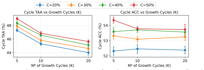
- Grow can reach high final accuracy during the editing procedure while Prune performs better when accuracy is averaged over the full training trajectory or when the final sparse network is retrained from scratch.
- Targeted changes to optimizer state, insertion location, selection criteria, or trainability improve the integration of new units but do not guarantee superior final subnetworks.
- In continual-learning settings that stress loss of plasticity, growth competes with other methods only when new units receive sufficient time to integrate into the existing trajectory.
- Growth must be evaluated as a time-sensitive optimization process rather than solely as an architecture-search operator.
Where Pith is reading between the lines
- Methods that temporarily shield new units from the full gradient flow or initialize them with separate optimizer states could reduce the integration delay observed in convolutional trunks.
- The timing of growth steps may matter more than their frequency, suggesting that scheduled pauses after each insertion could improve long-term stability in dynamic networks.
- If insertion stability proves central, growth operators might be combined with mechanisms that periodically reset or rescale gradients across the whole network to equalize signal strength.
Editorial analysis
A structured set of objections, weighed in public.
Referee Report
Summary. The paper claims that structural growth during training is not the inverse of pruning: growth inserts new units into an already-specialized optimization trajectory, causing newborn units to be forward-active but backward-starved (weaker gradients than incumbent units). This disadvantage is minor in small MLPs but pronounced in harder conv-net image-classification settings. Experiments compare Grow vs. Prune procedures, apply interventions on optimizer state/insertion/selection/trainability, and evaluate in continual-learning benchmarks; results indicate that improving newborn-unit integration aids adaptive performance but does not guarantee better final subnetworks, and Grow is competitive mainly when new units have time to integrate.
Significance. If the empirical distinctions hold, the work clarifies why growth-based structural plasticity can underperform relative to pruning in dynamic networks and underscores the need to treat growth as a time-sensitive optimization process rather than solely an architecture-search operator. The interventions on multiple factors (optimizer state, insertion timing, etc.) and the continual-learning evaluation provide concrete evidence that insertion stability matters for plasticity.
major comments (2)
- [Abstract] Abstract: the central attribution of gradient disadvantage specifically to insertion into a specialized trajectory (rather than optimizer state, scale, or initialization) rests on observational comparisons and interventions, yet the text provides no quantitative details on effect sizes, statistical tests, whether controls were applied uniformly in the main gradient-comparison runs, or whether scale was matched between Grow and Prune. This leaves open whether the observed backward starvation would disappear under identical optimizer state and scale but different insertion timing.
- [Abstract] Abstract / §4 (experiments): the claim that interventions targeting optimizer state, insertion, selection, and trainability improve integration but do not automatically produce better final subnetworks is load-bearing for the distinction between adaptive performance and final-subnetwork quality; without reported numbers on how uniformly these controls were applied or on the magnitude of gradient-signal recovery, the isolation of the insertion problem cannot be assessed.
minor comments (1)
- [Abstract] Abstract: the notation \textsc{Grow} and \textsc{Prune} is clear but the manuscript should define them explicitly on first use in the main text.
Simulated Author's Rebuttal
We thank the referee for the constructive comments, which highlight opportunities to strengthen the quantitative support for our claims. We address each major comment below and will incorporate the suggested clarifications in the revised manuscript.
read point-by-point responses
-
Referee: [Abstract] Abstract: the central attribution of gradient disadvantage specifically to insertion into a specialized trajectory (rather than optimizer state, scale, or initialization) rests on observational comparisons and interventions, yet the text provides no quantitative details on effect sizes, statistical tests, whether controls were applied uniformly in the main gradient-comparison runs, or whether scale was matched between Grow and Prune. This leaves open whether the observed backward starvation would disappear under identical optimizer state and scale but different insertion timing.
Authors: We agree that additional quantitative detail would improve clarity. The interventions in §4 do include matched-scale and optimizer-state controls (with newborn units inserted at different times into the same trajectory), and the gradient gap persists under those conditions, supporting the role of insertion timing. In the revision we will add a table of mean gradient magnitudes (with standard deviations over 5 seeds), report the results of paired statistical tests, and explicitly state that scale and optimizer state were matched in the primary gradient-comparison runs. We will also include a short paragraph quantifying how much of the gap remains after these controls. revision: yes
-
Referee: [Abstract] Abstract / §4 (experiments): the claim that interventions targeting optimizer state, insertion, selection, and trainability improve integration but do not automatically produce better final subnetworks is load-bearing for the distinction between adaptive performance and final-subnetwork quality; without reported numbers on how uniformly these controls were applied or on the magnitude of gradient-signal recovery, the isolation of the insertion problem cannot be assessed.
Authors: We acknowledge the need for explicit numbers. The experiments apply the four intervention types uniformly across the reported runs, and gradient-signal recovery is partial (typically 30-60 % of the incumbent-unit level) yet still yields improved online accuracy without corresponding gains in final subnetwork quality after retraining. In revision we will expand §4 with a table listing per-intervention gradient recovery percentages, confirm uniform application of controls, and add a sentence quantifying the dissociation between adaptive performance and final-subnetwork quality. revision: yes
Circularity Check
No circularity: purely empirical comparison with no derivation chain
full rationale
The paper presents an empirical study comparing Grow and Prune structural editing procedures on neural networks, focusing on gradient signals to newborn units and performance in image classification and continual learning. No mathematical derivations, first-principles predictions, fitted parameters renamed as outputs, or self-citation chains are present in the abstract or described content. All claims rest on experimental interventions and observations rather than any closed logical loop reducing results to inputs by construction. The work is self-contained as a set of controlled comparisons without invoking uniqueness theorems or ansatzes from prior self-work.
Axiom & Free-Parameter Ledger
read the original abstract
Standard deep-learning pipelines usually choose the network architecture before training and keep it fixed throughout optimization. In contrast, a model can also be adapted by editing its structure during training, for example by pruning existing hidden-neuron units or growing new ones. Although growth is appealing for adaptive and continual systems, we show that it is not simply the inverse of pruning. Pruning selects among units that have participated in training from the start, whereas growth inserts new units into an already specialized optimization trajectory. We isolate this insertion problem and show that newborn units are often forward-active but backward-starved: they participate in the forward computation, yet receive much weaker gradient signal than incumbent units. This disadvantage is minor in small MLP benchmarks, but becomes clear in harder image-classification settings with a convolutional trunk. In these settings, \textsc{Grow} can achieve high final accuracy during the structural-editing procedure, while \textsc{Prune} is stronger when performance is averaged over the training trajectory or when the final sparse network is retrained from scratch. Interventions targeting optimizer state, insertion, selection, and trainability show that improving the integration of newborn units can improve adaptive performance, but does not automatically produce better final subnetworks. In continual-learning benchmarks stressing plasticity loss, \textsc{Grow} becomes competitive mainly when new units have enough time to integrate. Together, these results suggest that \textsc{Grow} should be evaluated not only as an architecture-search operator, but as a time-sensitive optimization process whose success depends on insertion stability.
Figures




Reference graph
Works this paper leans on
-
[1]
Asadi, K., Fakoor, R., and Sabach, S. (2023). Resetting the optimizer in deep rl: An empirical study.Advances in Neural Information Processing Systems, 36:72284–72324
2023
- [2]
-
[3]
Bellec, G., Kappel, D., Maass, W., and Legenstein, R. (2017). Deep rewiring: Training very sparse deep networks.arXiv preprint arXiv:1711.05136
work page internal anchor Pith review Pith/arXiv arXiv 2017
-
[4]
Cai, Z., Sener, O., and Koltun, V. (2021). Online continual learning with natural distribution shifts: An empirical study with visual data. InProceedings of the IEEE/CVF international conference on computer vision, pages 8281–8290
2021
-
[5]
Chen, T., Goodfellow, I., and Shlens, J. (2016). Net2net: Accelerating learning via knowledge transfer. InICLR
2016
-
[6]
Cheney, N., Schrimpf, M., and Kreiman, G. (2017). On the robustness of convolutional neural networks to internal architecture and weight perturbations.arXiv preprint arXiv:1703.08245
work page internal anchor Pith review Pith/arXiv arXiv 2017
-
[7]
Dai, X., Yin, H., and Jha, N. K. (2019). Nest: A neural network synthesis tool based on a grow-and-prune paradigm.IEEE Transactions on Computers, 68(10):1487–1497
2019
-
[8]
Dettmers, T. and Zettlemoyer, L. (2019). Sparse networks from scratch: Faster training without losing performance.arXiv preprint arXiv:1907.04840
-
[9]
F., Lan, Q., Rahman, P., Mahmood, A
Dohare, S., Hernandez-Garcia, J. F., Lan, Q., Rahman, P., Mahmood, A. R., and Sutton, R. S. (2024). Loss of plasticity in deep continual learning.Nature, 632:768—774
2024
-
[10]
Evci, U., Gale, T., Menick, J., Sampedro, P., Lorch, E., and Sohl-Dickstein, J. (2020). Rigging the lottery: Making all tickets winners. InNeurIPS
2020
-
[11]
Evci, U., van Merrienboer, B., Unterthiner, T., Pedregosa, F., and Vladymyrov, M. (2022). Gradmax: Growing neural networks using gradient information. InInternational Conference on Learning Representations
2022
-
[12]
PathNet: Evolution Channels Gradient Descent in Super Neural Networks
Fernando, C., Banarse, D., Blundell, C., Zwols, Y., Ha, D., Rusu, A. A., Pritzel, A., and Wierstra, D. (2017). Pathnet: Evolution channels gradient descent in super neural networks.arXiv preprint arXiv:1701.08734
work page internal anchor Pith review Pith/arXiv arXiv 2017
-
[13]
The Lottery Ticket Hypothesis: Finding Sparse, Trainable Neural Networks
Frankle, J. and Carbin, M. (2018). The lottery ticket hypothesis: Finding sparse, trainable neural networks.arXiv preprint arXiv:1803.03635
work page internal anchor Pith review Pith/arXiv arXiv 2018
-
[14]
K., Roy, D
Frankle, J., Dziugaite, G. K., Roy, D. M., and Carbin, M. (2019). Stabilizing the lottery ticket hypothesis.arXiv: Learning
2019
-
[15]
A., Prabhu, A., Torr, P
Ghunaim, Y., Bibi, A., Alhamoud, K., Alfarra, M., Al Kader Hammoud, H. A., Prabhu, A., Torr, P. H., and Ghanem, B. (2023). Real-time evaluation in online continual learning: A new hope. InProceedings of the IEEE/CVF conference on computer vision and pattern recognition, pages 11888–11897
2023
-
[16]
An Empirical Investigation of Catastrophic Forgetting in Gradient-Based Neural Networks
Goodfellow, I. J., Mirza, M., Xiao, D., Courville, A., and Bengio, Y. (2013). An empirical investigation of catastrophic forgetting in gradient-based neural networks.arXiv preprint arXiv:1312.6211. 10
work page internal anchor Pith review Pith/arXiv arXiv 2013
-
[17]
Gordon, A., Eban, E., Nachum, O., Chen, B., Wu, H., Yang, T.-J., and Choi, E. (2018). Morphnet: Fast & simple resource-constrained structure learning of deep networks. InProceedings of the IEEE conference on computer vision and pattern recognition, pages 1586–1595
2018
-
[18]
Han, S., Mao, H., and Dally, W. J. (2015a). Deep compression: Compressing deep neural net- works with pruning, trained quantization and huffman coding.arXiv preprint arXiv:1510.00149
work page internal anchor Pith review Pith/arXiv arXiv
-
[19]
Han, S., Pool, J., Tran, J., and Dally, W. (2015b). Learning both weights and connections for efficient neural network.Advances in neural information processing systems, 28
-
[20]
Kang, H., Mina, R. J. L., Madjid, S. R. H., Yoon, J., Hasegawa-Johnson, M., Hwang, S. J., and Yoo, C. D. (2022). Forget-free continual learning with winning subnetworks. In Chaudhuri, K., Jegelka, S., Song, L., Szepesvari, C., Niu, G., and Sabato, S., editors,Proceedings of the 39th International Conference on Machine Learning, volume 162 ofProceedings of...
2022
-
[21]
Kingma, D. P. and Ba, J. (2014). Adam: A method for stochastic optimization.arXiv preprint arXiv:1412.6980
work page internal anchor Pith review Pith/arXiv arXiv 2014
-
[22]
Krizhevsky, A. (2009). Learning multiple layers of features from tiny images. InUniversity of Toronto Technical Report
2009
- [23]
- [24]
-
[25]
Lecun, Y., Bottou, L., Bengio, Y., and Haffner, P. (1998). Gradient-based learning applied to document recognition.Proceedings of the IEEE, 86(11):2278–2324
1998
-
[26]
Li, X., Zhou, Y., Wu, T., Socher, R., and Xiong, C. (2019). Learn to grow: A continual structure learning framework for overcoming catastrophic forgetting. InInternational conference on machine learning, pages 3925–3934. PMLR
2019
-
[27]
Activation Function Design Sustains Plasticity in Continual Learning
Lillo, L. and Cheney, N. (2025). Activation function design sustains plasticity in continual learning.arXiv preprint arXiv:2509.22562
work page internal anchor Pith review Pith/arXiv arXiv 2025
-
[28]
A., Pascanu, R., and Dabney, W
Lyle, C., Zheng, Z., Nikishin, E., Pires, B. A., Pascanu, R., and Dabney, W. (2023). Understanding plasticity in neural networks. InInternational Conference on Machine Learning, pages 23190– 23211. PMLR
2023
-
[29]
Mallya, A., Davis, D., and Lazebnik, S. (2018). Piggyback: Adapting a single network to multiple tasks by learning to mask weights. InProceedings of the European conference on computer vision (ECCV), pages 67–82
2018
-
[30]
and Lazebnik, S
Mallya, A. and Lazebnik, S. (2018). Packnet: Adding multiple tasks to a single network by iterative pruning. InProceedings of the IEEE conference on Computer Vision and Pattern Recognition, pages 7765–7773
2018
-
[31]
Miconi, T. (2016). Neural networks with differentiable structure.arXiv preprint arXiv:1606.06216
work page internal anchor Pith review Pith/arXiv arXiv 2016
-
[32]
Mocanu, D. C. et al. (2018). Scalable training of artificial neural networks with adaptive sparse connectivity. InAAAI. 11
2018
- [33]
- [34]
-
[35]
On the Convergence of Adam and Beyond
Reddi, S. J., Kale, S., and Kumar, S. (2019). On the convergence of adam and beyond.arXiv preprint arXiv:1904.09237
work page internal anchor Pith review Pith/arXiv arXiv 2019
-
[36]
C., and Fei-Fei, L
Russakovsky, O., Deng, J., Su, H., Krause, J., Satheesh, S., Ma, S., Huang, Z., Karpathy, A., Khosla, A., Bernstein, M., Berg, A. C., and Fei-Fei, L. (2015). ImageNet Large Scale Visual Recognition Challenge.International Journal of Computer Vision (IJCV), 115(3):211–252
2015
-
[37]
Rusu, A. A., Rabinowitz, N. C., Desjardins, G., Soyer, H., Kirkpatrick, J., Kavukcuoglu, K., Pascanu, R., and Hadsell, R. (2016). Progressive neural networks.arXiv preprint arXiv:1606.04671
work page internal anchor Pith review Pith/arXiv arXiv 2016
-
[38]
Wei, T., Wang, C., Rui, Y., and Chen, C. W. (2016). Network morphism. InProceedings of the 33rd International Conference on Machine Learning (ICML)
2016
-
[39]
Wu, L., Liu, B., Stone, P., and Liu, Q. (2020). Firefly neural architecture descent: a general approach for growing neural networks.Advances in neural information processing systems, 33:22373–22383
2020
-
[40]
Wu, L., Wang, D., and Liu, Q. (2019). Splitting steepest descent for growing neural architectures. Advances in neural information processing systems, 32
2019
-
[41]
Xiao, H., Rasul, K., and Vollgraf, R. (2017). Fashion-mnist: a novel image dataset for bench- marking machine learning algorithms.arXiv preprint arXiv:1708.07747
work page internal anchor Pith review Pith/arXiv arXiv 2017
-
[42]
Xiong, R., Yang, Y., He, D., Zheng, K., Zheng, S., Xing, C., Zhang, H., Lan, Y., Wang, L., and Liu, T. (2020). On layer normalization in the transformer architecture. InInternational conference on machine learning, pages 10524–10533. PMLR
2020
- [43]
-
[44]
Yoon, J., Yang, E., Lee, J., and Hwang, S. J. (2017). Lifelong learning with dynamically expand- able networks.arXiv preprint arXiv:1708.01547
work page internal anchor Pith review Pith/arXiv arXiv 2017
-
[45]
You, Y., Li, J., Reddi, S., Hseu, J., Kumar, S., Bhojanapalli, S., Song, X., Demmel, J., Keutzer, K., and Hsieh, C.-J. (2019). Large batch optimization for deep learning: Training bert in 76 minutes. arXiv preprint arXiv:1904.00962
work page internal anchor Pith review Pith/arXiv arXiv 2019
-
[46]
Yuan, X., Savarese, P., and Maire, M. (2023). Accelerated training via incrementally growing neural networks using variance transfer and learning rate adaptation.Advances in Neural Information Processing Systems, 36:16673–16692
2023
- [47]
-
[48]
C., Dvornek, N., Papademetris, X., and Duncan, J
Zhuang, J., Tang, T., Ding, Y., Tatikonda, S. C., Dvornek, N., Papademetris, X., and Duncan, J. (2020). Adabelief optimizer: Adapting stepsizes by the belief in observed gradients.Advances in neural information processing systems, 33:18795–18806. 12 Submission Checklist
2020
-
[49]
For all authors. . . (a) Do the main claims made in the abstract and introduction accurately reflect the paper’s contributions and scope? [Yes] The abstract and introduction accurately reflect the paper’s contributions and scope. (b) Did you describe the limitations of your work? [Yes] We discuss limitations, including the restricted architectural setting...
2022
-
[50]
If you ran experiments. . . (a) Did you use the same evaluation protocol for all methods being compared (e.g., same benchmarks, data (sub)sets, available resources, etc.)? [Yes] All compared methods use the same datasets, architectures, training budgets, evaluation checkpoints, and compactness targets unless explicitly stated. (b) Did you specify all the ...
-
[51]
With respect to the code used to obtain your results. . . (a) Did you include the code, data, and instructions needed to reproduce the main experimental results, including all dependencies (e.g., requirements.txt with explicit versions), random seeds, an instructive README with installation instructions, and execution commands (ei- ther in the supplementa...
-
[52]
(a) Did you cite the creators of used assets? [Yes] We cite the creators of all datasets, algorithms, and software assets used
If you used existing assets (e.g., code, data, models). . . (a) Did you cite the creators of used assets? [Yes] We cite the creators of all datasets, algorithms, and software assets used. (b) Did you discuss whether and how consent was obtained from people whose data you’re using/curating if the license requires it? [N/A] We use standard public benchmark ...
-
[53]
(a) Did you mention the license of the new assets (e.g., as part of your code submission)? [Yes] The license for released code and assets is specified
If you created/released new assets (e.g., code, data, models). . . (a) Did you mention the license of the new assets (e.g., as part of your code submission)? [Yes] The license for released code and assets is specified. (b) Did you include the new assets either in the supplemental material or as aurl(to, e.g., GitHub or Hugging Face)? [Yes] The released as...
-
[54]
(a) Did you include the full text of instructions given to participants and screenshots, if appli- cable? [No] No crowdsourcing or human-subject experiments were conducted
If you used crowdsourcing or conducted research with human subjects. . . (a) Did you include the full text of instructions given to participants and screenshots, if appli- cable? [No] No crowdsourcing or human-subject experiments were conducted. (b) Did you describe any potential participant risks, with links to institutional review board (irb) approvals,...
-
[55]
If you included theoretical results. . . (a) Did you state the full set of assumptions of all theoretical results? [No] The paper does not present theoretical results. (b) Did you include complete proofs of all theoretical results? [No] The paper does not present theoretical results. 15 A Datasets, Benchmarks and Hyperparameters A.1 Datasets and Benchmark...
discussion (0)
Sign in with ORCID, Apple, or X to comment. Anyone can read and Pith papers without signing in.