Global analysis of a minimally extended scotogenic model
Pith reviewed 2026-07-01 07:15 UTC · model grok-4.3
The pith
A numerical scan of the minimally extended scotogenic model identifies viable fermionic dark matter masses between 120 and 350 GeV while the DESI BAO bound excludes the inverted neutrino hierarchy.
A machine-rendered reading of the paper's core claim, the machinery that carries it, and where it could break.
Core claim
A numerical scan of the minimally extended scotogenic model that incorporates vacuum-stability and perturbativity requirements together with flavor and electroweak precision observables yields viable parameter space in which the fermionic dark-matter candidate has mass 120-350 GeV, the CP-odd scalar has mass 350-600 GeV, the oblique parameters lie within reach of forthcoming measurements, the Z to invisible branching ratio is compatible with the world average at the 3 sigma level and favored by recent ATLAS data at the 3 sigma level, and the inverted neutrino mass hierarchy is excluded if the DESI BAO bound is confirmed.
What carries the argument
The minimally extended scotogenic model, an extension of the Standard Model by additional scalar and fermionic fields that generates neutrino masses radiatively at one loop while supplying a stable dark-matter candidate and addressing vacuum instability.
If this is right
- The inverted neutrino hierarchy is ruled out once the DESI BAO bound is adopted.
- Projected values of the oblique parameters fall inside the sensitivity of next-generation precision electroweak measurements.
- Direct searches for fermionic dark matter should target the 120-350 GeV interval.
- The CP-odd scalar is restricted to the 350-600 GeV window by the combined constraints.
- The predicted Z to invisible width remains compatible with existing data at the 3 sigma level.
Where Pith is reading between the lines
- The narrow mass windows narrow the target range for upcoming direct-detection and collider searches for both the dark-matter fermion and the additional scalar.
- Preference for the normal hierarchy under DESI data aligns the model with independent cosmological indications that already favor normal ordering.
- If future measurements tighten the oblique-parameter bounds without finding the predicted shifts, the viable parameter space would shrink further.
- The compatibility with the ATLAS Z invisible result suggests that modest improvements in invisible-width precision could begin to discriminate among scotogenic variants.
Load-bearing premise
The chosen set of flavor, electroweak, vacuum-stability, and perturbativity constraints is assumed to be sufficient to capture all relevant restrictions on the model's parameter space.
What would settle it
A confirmed measurement of the inverted neutrino hierarchy that remains consistent with the DESI BAO bound, or a dark-matter particle whose mass lies outside the 120-350 GeV window while satisfying all other listed observables, would falsify the scan results.
Figures





read the original abstract
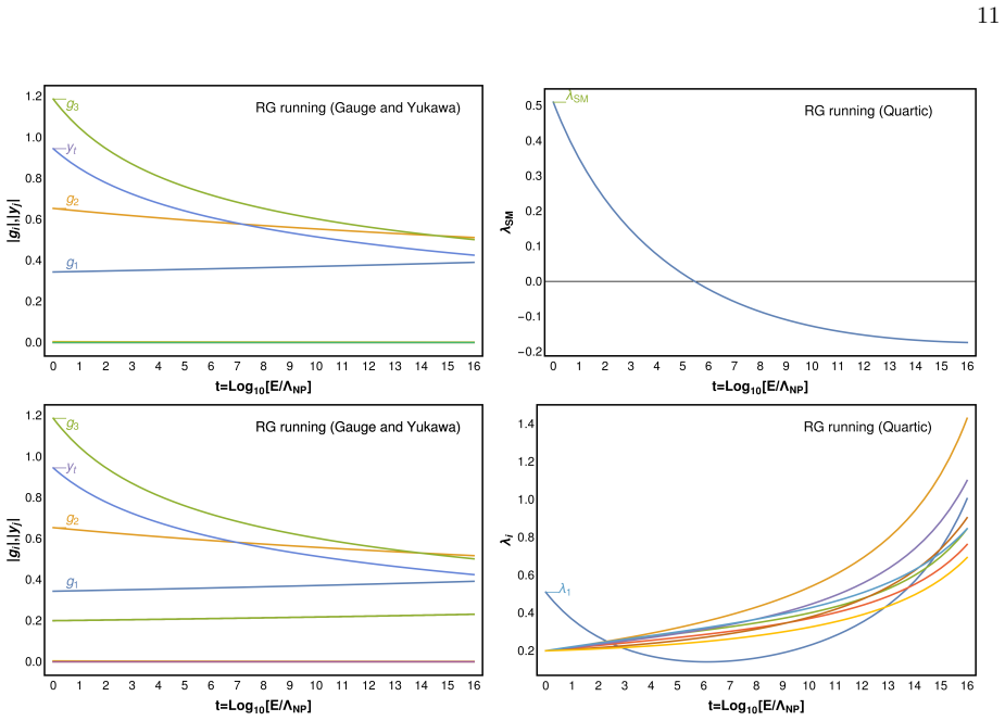
We perform a global analysis of a minimally extended scotogenic model motivated by observed non-zero neutrino masses, viable dark matter (DM) candidates, and the instability of the Standard Model (SM) vacuum at high-energies. We examine the bounded-from-below conditions, vacuum stability, and RG-driven perturbativity bounds arising from the extended scalar sector, alongside a comprehensive set of flavor and electroweak (EW) precision observables - including the muon anomalous magnetic moment $\Delta a_{\mu}$, the radiative decays $\ell_{\alpha} \rightarrow \ell_{\beta} \gamma$ and $\ell_{\alpha} \rightarrow 3\ell_{\beta}$, and the $\mu \rightarrow e$ conversion rate, the oblique parameters, and leptonic decays of $Z$ and $H$ bosons. A numerical scan reveals four notable features: the DESI BAO bound would rule out the inverted hierarchy if confirmed by other experiments; the oblique parameters are projected to be within the reach of future precision measurements; the viable fermionic DM candidate mass lies in the range $120-350 \operatorname{GeV}$, while the CP-odd scalar is constrained to $350-600 \operatorname{GeV}$; and our result on $Z \rightarrow \operatorname{Invisible}$ is compatible with the world average at the $3\sigma$ level and is favored by the recent ATLAS measurement at the $3\sigma$ level.
Editorial analysis
A structured set of objections, weighed in public.
Referee Report
Summary. The manuscript performs a global analysis of a minimally extended scotogenic model, incorporating additional scalars and fermions to generate neutrino masses, provide dark matter candidates, and address SM vacuum instability. Constraints from bounded-from-below conditions, vacuum stability, RG perturbativity, flavor observables (including Δa_μ, radiative decays, μ→e conversion), oblique parameters, and leptonic Z/H decays are applied via a numerical scan over scalar potential couplings, masses, and Yukawa couplings. The scan yields four reported features: DESI BAO data would exclude inverted neutrino hierarchy; oblique parameters lie within future experimental reach; viable fermionic DM mass in 120-350 GeV and CP-odd scalar in 350-600 GeV; and Z→invisible width compatible with world average at 3σ and favored by recent ATLAS data at 3σ.
Significance. If the scan methodology and constraint implementation are robust, the results supply concrete, testable mass windows for DM and scalar states, a potential hierarchy discriminator via BAO, and indications that precision EW observables can probe the model, strengthening the phenomenological case for minimally extended scotogenic scenarios beyond existing literature.
minor comments (3)
- The abstract states that a numerical scan was performed but provides no information on methodology, prior ranges, convergence checks, or post-hoc cuts. The full manuscript should include a dedicated subsection (e.g., §3 or §4) detailing the scan procedure, parameter ranges, and validation to allow reproduction of the quoted mass windows and 3σ statements.
- The four notable features are presented as direct outputs of the scan; clarify in the results section whether any (e.g., Z invisible width) constitute genuine predictions or are by construction within the fitted observables.
- Minor notation inconsistency: the abstract uses “Z → Invisible” while the text likely employs standard Γ(Z→inv); ensure uniform notation throughout.
Simulated Author's Rebuttal
We thank the referee for their careful reading of the manuscript and for the positive assessment, including the recommendation for minor revision. The referee summary accurately captures the scope and main findings of our global analysis. No major comments were raised that require point-by-point rebuttal.
Circularity Check
No significant circularity identified
full rationale
The paper performs a standard global numerical scan of a scotogenic model extension, imposing external constraints from vacuum stability, perturbativity, flavor observables, EW precision data, and DM requirements. The reported features (mass ranges, hierarchy exclusion under DESI, oblique parameter projections, Z invisible width compatibility) are direct outputs of this scan applied to the chosen observables; none reduce by construction to the inputs via self-definition, renaming, or self-citation chains. The derivation remains self-contained against the listed external benchmarks with no load-bearing internal reduction exhibited.
Axiom & Free-Parameter Ledger
free parameters (2)
- scalar potential couplings and masses
- Yukawa couplings to new fermions
axioms (2)
- domain assumption The Standard Model vacuum instability is cured by the new scalars without introducing new instabilities at higher scales.
- domain assumption All relevant constraints are captured by the listed flavor, EW precision, and vacuum-stability observables.
Reference graph
Works this paper leans on
-
[1]
Generate an initial point in the parameter space yielding a finite log likelihood value, defined as lnL= X i lnL i =− X i Opred i − Oexp i 2 2σ2 i ,(49) whereO pred i andO exp i denote the predicted and experimental values of thei-th observable, respectively, andσ i is the corresponding 1σuncertainty
-
[2]
Propose a candidate point sampled from a Gaussian distribution centered on the current point
-
[3]
Evaluate theχ 2 value at the candidate point and determine whether to accept or reject it according to the Metropolis–Hastings criterion
-
[4]
Repeat steps 2–4 until the chain reaches sufficient convergence. The primary observables driving the MCMC algorithm are the SM Higgs boson mass at one-loop level and the relic density, whose experimental values are taken asm h = 125.20±0.11 GeV [71] and Ωh 2 = 0.120±0.012 of Equation 13, respectively. The ranges of the input parameters are listed in Table...
-
[5]
For the sixth diagram, an equivalent diagram with reversed charge flow is included
Photon self-energy The diagrams contributing to the photon SE in this work are seen in Figure 15: The counter- term for the photon self-energy in the scotogenic model is given in Equation B1: δZAA =− ∂ΣAA T p2 ∂p2 p2=0 = e2(s2 w −1) 144c2w(D−1)π 2 " Nc 3X i=1 (2D−4)B 0(0, m2 di, m2 di) + 8m2 di DB0(0, m2 di, m2 di) 32 γ γ G+,H + γ γ W + γ γ ui,d i,e i ui,...
-
[6]
3.Zself-energy FromZSE, the tadpole contributions start to appear
Photon-Zself-energy The diagrams contributing to the photon-ZSE in this work are seen in Figure 16: The counter- 33 terms for the photon-Zself-energy in the scotogenic model is given in Equation B2: δZZA = 2 M 2 Z ΣAZ T (0) =− e2cw B0 0, M2 W , M2 W 4π2sw , δZAZ =−2 Re ΣAZ T M 2 Z M 2 Z = e2 144c w(1−D)M 2 Zπ2sw " + 36M2 H ± 1−2s 2 w B0 0, M2 H ±, M2 H ± ...
-
[7]
∂Σh1h1 p2 ∂p2 # p2=m2 h1 ,(B8) δZh1h2 = 2 m2 h1 −m 2 h2 Re Σh1h2 m2 h2 ,(B9) δZh2h1 = 2 m2 h2 −m 2 h1 Re Σh1h2 m2 h1 ,(B10) δZh2h2 =−Re
Scalar self-energy The diagrams contributing to the scalar tadpole and SE are seen in Figure 21 and Figure 22. Since the scalar sector is extended, the mass and field CTs are defined as follows. In what follows, 43 hi hj ul, dl, el hk hi hj χl hk hi hj hl,a l,ηR,I hk hi hj G+, H+ hk hi hj ηZ,η± W hk hi hj Z hk hi hj W + hk Figure 21: Feynman diagrams cont...
-
[8]
Charged lepton self-energy The diagrams contributing to the chaged lepton tadpole and SE are seen in Figure 23 and Figure 24. Following [75], the charged lepton propagator - with incoming and outgoing leptons indexed byjandi, respectively - can be decomposed in terms of the projected self-energies with distinct Dirac structures as: Γf ij (p) =iδ ij /p−m i...
-
[9]
Consequently, only SE contributions arise
Neutrino self-energy In the neutrino sector, tadpole contributions are absent in both the SM and the BSM model, as there is noh i −v−vvertex. Consequently, only SE contributions arise. The diagrams contributing to the neutrino SE in the scotogenic model and the SM are shown in Figures 25 and 26, respectively. The diagonal and off-diagonal CTs for the neut...
-
[10]
The scalar potential then reduces to: V4 (a=d=e= 0) = 1 4 p λ2b− p λ6c 2 + 1 2 p λ2λ6 +λ 8 bc,(C5) which gives rise to the first condition: λ8 + 1 2 p λ2λ6 >0 (C6) 47
a=0 Whena= 0, the parametersdandevanish as a consequence of the inequality C3. The scalar potential then reduces to: V4 (a=d=e= 0) = 1 4 p λ2b− p λ6c 2 + 1 2 p λ2λ6 +λ 8 bc,(C5) which gives rise to the first condition: λ8 + 1 2 p λ2λ6 >0 (C6) 47
-
[11]
V4 (b=d=e= 0) = 1 4 p λ1a− p λ6c 2 + 1 2 p λ1λ6 +λ 7 ac,(C7) which yields the second condition: λ7 + 1 2 p λ1λ6 >0 (C8)
b=0 Whenb= 0, the derivation follows analogously to the previous casea= 0. V4 (b=d=e= 0) = 1 4 p λ1a− p λ6c 2 + 1 2 p λ1λ6 +λ 7 ac,(C7) which yields the second condition: λ7 + 1 2 p λ1λ6 >0 (C8)
-
[12]
First, we take the direction defined byd=e= 0
c=0 Whenc= 0, the reduced scalar potential is: V4 (c= 0) = 1 4 p λ1a− p λ2b 2 + 1 2 p λ1λ2 +λ 3 ab+λ 4 d2 +e 2 + 1 2 λ5 d2 −e 2 .(C9) To derive the BFB conditions, we need to examine additional field directions. First, we take the direction defined byd=e= 0. The scalar potential further reduces to: V4 (c=d=e= 0) = 1 4 p λ1a− p λ2b 2 + 1 2 p λ1λ2 +λ 3 ab,(...
-
[13]
(C14) 48 In this direction, the inequality can be rewritten in terms of the parametercalone: ab≥d 2 +e 2 λ6√λ1λ2 c2 ≥d 2 +e 2
a= p λ6/λ1c, b= p λ6/λ2c With this direction, the scalar potential reduces to: V4 a= r λ6 λ1 c, b= r λ6 λ2 c ! = 3 4 λ6 + λ3λ6√λ1λ2 +λ 7 r λ6 λ1 +λ 8 r λ6 λ2 ! c2 +λ 4 d2 +e 2 + 1 2 λ5 d2 −e 2 ≡λ ac2 +λ 4 d2 +e 2 + 1 2 λ5 d2 −e 2 . (C14) 48 In this direction, the inequality can be rewritten in terms of the parametercalone: ab≥d 2 +e 2 λ6√λ1λ2 c2 ≥d 2 +e 2...
-
[14]
Standard Model The SM RGEs are as follows: β(1) (g1) = 41 10 g3 1 (D2) β(1) (g2) =− 19 6 g3 2 (D3) β(1) (g3) =−7g 3 3 (D4) β(1)(y(i,j) u ) = −17 20 g2 1 − 9 4 g2 2 −8g 2 3 + 3 Tr h yuy† u i + 3 Tr h ydy† d i + Tr h yey† e i y(i,j) u − 3 2 yuy† dyd −y uy† uyu (i,j) (D5) β(1)(y(i,j) d ) = 1 4 −g2 1 −9g 2 2 −32g 2 3 + 12 Tr h ydy† d i + 4 Tr h yey† e i + 12 ...
-
[15]
Scotogenic Model The Scotogenic RGEs are as follows: β(1) (g1) = 21 5 g3 1 (D9) β(1) (g2) =−3g 3 2 (D10) β(1) (g3) =−7g 3 3 (D11) β(1)(y(i,j) u ) = −17 20 g2 1 − 9 4 g2 2 −8g 2 3 + 3 Tr h ydy† d i + Tr h yey† e i + 3 Tr h yuy† u i y(i,j) u − 3 2 yuy† dyd −y uy† uyu (i,j) (D12) β(1)(y(i,j) d ) = 1 4 −g2 1 −9g 2 2 −32g 2 3 + 12 Tr h ydy† d i + 4 Tr h yey† e...
-
[16]
Verifiable Radiative Seesaw Mechanism of Neutrino Mass and Dark Matter
E. Ma, Phys. Rev. D73, 077301 (2006), hep-ph/0601225
work page internal anchor Pith review Pith/arXiv arXiv 2006
- [17]
-
[18]
Planck 2018 results. VI. Cosmological parameters
N. Aghanim et al. (Planck), Astron. Astrophys.641, A6 (2020), [Erratum: Astron.Astrophys. 652, C4 (2021)], 1807.06209
work page internal anchor Pith review Pith/arXiv arXiv 2020
-
[19]
Fleischer and F
J. Fleischer and F. Jegerlehner, Phys. Rev. D23, 2001 (1981)
2001
-
[20]
A. A. Markov, inDynamic Probabilistic Systems, Volume 1: Markov Chains, edited by R. Howard (John Wiley and Sons, 1971), reprinted in Appendix B
1971
-
[21]
The anomalous magnetic moment of the muon in the Standard Model
T. Aoyama et al., Phys. Rept.887, 1 (2020), 2006.04822
work page internal anchor Pith review Pith/arXiv arXiv 2020
-
[22]
The anomalous magnetic moment of the muon in the Standard Model: an update
R. Aliberti et al., Phys. Rept.1143, 1 (2025), 2505.21476
work page internal anchor Pith review Pith/arXiv arXiv 2025
-
[23]
J. A. Casas and A. Ibarra, Nucl. Phys. B618, 171 (2001), hep-ph/0103065
work page internal anchor Pith review Pith/arXiv arXiv 2001
-
[24]
NuFit-6.0: Updated global analysis of three-flavor neutrino oscillations
I. Esteban, M. C. Gonzalez-Garcia, M. Maltoni, I. Martinez-Soler, J. P. Pinheiro, and T. Schwetz, JHEP12, 216 (2024), 2410.05380
work page internal anchor Pith review Pith/arXiv arXiv 2024
-
[25]
F. Boudjema, G. Drieu La Rochelle, and A. Mariano, Phys. Rev. D89, 115020 (2014), 1403.7459
work page internal anchor Pith review Pith/arXiv arXiv 2014
-
[26]
J. Harz, B. Herrmann, M. Klasen, K. Kovarik, and P. Steppeler, Phys. Rev. D93, 114023 (2016), 1602.08103
work page internal anchor Pith review Pith/arXiv arXiv 2016
-
[27]
G. Alguero, G. Belanger, F. Boudjema, S. Chakraborti, A. Goudelis, S. Kraml, A. Mjallal, and A. Pukhov, Comput. Phys. Commun.299, 109133 (2024), 2312.14894
-
[28]
Investigating the near-criticality of the Higgs boson
D. Buttazzo, G. Degrassi, P. P. Giardino, G. F. Giudice, F. Sala, A. Salvio, and A. Strumia, JHEP12, 089 (2013), 1307.3536
work page internal anchor Pith review Pith/arXiv arXiv 2013
-
[29]
J. E. Camargo-Molina and B. O’Leary (2014), https://github.com/JoseEliel/VevaciousPlusPlus
2014
-
[30]
J. E. Camargo-Molina, B. O’Leary, W. Porod, and F. Staub, Eur. Phys. J. C73, 2588 (2013), 1307.1477
work page internal anchor Pith review Pith/arXiv arXiv 2013
- [31]
-
[32]
Generating Feynman Diagrams and Amplitudes with FeynArts 3
T. Hahn, Comput. Phys. Commun.140, 418 (2001), hep-ph/0012260
work page internal anchor Pith review Pith/arXiv arXiv 2001
-
[33]
FeynCalc 9.3: New features and improvements
V. Shtabovenko, R. Mertig, and F. Orellana, Comput. Phys. Commun.256, 107478 (2020), 2001.04407
work page internal anchor Pith review Pith/arXiv arXiv 2020
-
[34]
New Developments in FeynCalc 9.0
V. Shtabovenko, R. Mertig, and F. Orellana, Comput. Phys. Commun.207, 432 (2016), 1601.01167
work page internal anchor Pith review Pith/arXiv arXiv 2016
-
[35]
Krause, Master’s thesis, KIT, Karlsruhe, TP (2016)
M. Krause, Master’s thesis, KIT, Karlsruhe, TP (2016)
2016
-
[36]
W. Porod, Comput. Phys. Commun.153, 275 (2003), hep-ph/0301101
work page internal anchor Pith review Pith/arXiv arXiv 2003
-
[37]
SPheno 3.1: extensions including flavour, CP-phases and models beyond the MSSM
W. Porod and F. Staub, Comput. Phys. Commun.183, 2458 (2012), 1104.1573
work page internal anchor Pith review Pith/arXiv arXiv 2012
-
[38]
Refinements in electroweak contributions to the muon anomalous magnetic moment
A. Czarnecki, W. J. Marciano, and A. Vainshtein, Phys. Rev. D67, 073006 (2003), [Erratum: Phys.Rev.D 73, 119901 (2006)], hep-ph/0212229
work page internal anchor Pith review Pith/arXiv arXiv 2003
-
[39]
Hadronic light-by-light scattering contribution to the muon anomalous magnetic moment revisited
K. Melnikov and A. Vainshtein, Phys. Rev. D70, 113006 (2004), hep-ph/0312226
work page internal anchor Pith review Pith/arXiv arXiv 2004
-
[40]
Complete Tenth-Order QED Contribution to the Muon g-2
T. Aoyama, M. Hayakawa, T. Kinoshita, and M. Nio, Phys. Rev. Lett.109, 111808 (2012), 1205.5370
work page internal anchor Pith review Pith/arXiv arXiv 2012
-
[41]
A. Kurz, T. Liu, P. Marquard, and M. Steinhauser, Phys. Lett. B734, 144 (2014), 1403.6400
work page internal anchor Pith review Pith/arXiv arXiv 2014
-
[42]
Reevaluation of the Hadronic Contributions to the Muon g-2 and to alpha(MZ)
M. Davier, A. Hoecker, B. Malaescu, and Z. Zhang, Eur. Phys. J. C71, 1515 (2011), [Erratum: Eur.Phys.J.C 72, 1874 (2012)], 1010.4180
work page internal anchor Pith review Pith/arXiv arXiv 2011
-
[43]
The electroweak contributions to (g-2)_\mu\ after the Higgs boson mass measurement
C. Gnendiger, D. St¨ ockinger, and H. St¨ ockinger-Kim, Phys. Rev. D88, 053005 (2013), 1306.5546
work page internal anchor Pith review Pith/arXiv arXiv 2013
-
[44]
Remarks on higher-order hadronic corrections to the muon g-2
G. Colangelo, M. Hoferichter, A. Nyffeler, M. Passera, and P. Stoffer, Phys. Lett. B735, 90 (2014), 1403.7512
work page internal anchor Pith review Pith/arXiv arXiv 2014
-
[45]
M. Davier, A. Hoecker, B. Malaescu, and Z. Zhang, Eur. Phys. J. C77, 827 (2017), 1706.09436
work page internal anchor Pith review Pith/arXiv arXiv 2017
-
[46]
Pseudoscalar-pole contribution to the $(g_{\mu}-2)$: a rational approach
P. Masjuan and P. Sanchez-Puertas, Phys. Rev. D95, 054026 (2017), 1701.05829
work page internal anchor Pith review Pith/arXiv arXiv 2017
-
[47]
Dispersion relation for hadronic light-by-light scattering: two-pion contributions
G. Colangelo, M. Hoferichter, M. Procura, and P. Stoffer, JHEP04, 161 (2017), 1702.07347
work page internal anchor Pith review Pith/arXiv arXiv 2017
-
[48]
Dispersion relation for hadronic light-by-light scattering: pion pole
M. Hoferichter, B.-L. Hoid, B. Kubis, S. Leupold, and S. P. Schneider, JHEP10, 141 (2018), 1808.04823
work page internal anchor Pith review Pith/arXiv arXiv 2018
-
[49]
The muon $g-2$ and $\alpha(M_Z^2)$: a new data-based analysis
A. Keshavarzi, D. Nomura, and T. Teubner, Phys. Rev. D97, 114025 (2018), 1802.02995
work page internal anchor Pith review Pith/arXiv arXiv 2018
-
[50]
Two-pion contribution to hadronic vacuum polarization
G. Colangelo, M. Hoferichter, and P. Stoffer, JHEP02, 006 (2019), 1810.00007
work page internal anchor Pith review Pith/arXiv arXiv 2019
-
[51]
M. Hoferichter, B.-L. Hoid, and B. Kubis, JHEP08, 137 (2019), 1907.01556
- [52]
-
[53]
A. Keshavarzi, D. Nomura, and T. Teubner, Phys. Rev. D101, 014029 (2020), 1911.00367
-
[54]
A. G´ erardin, H. B. Meyer, and A. Nyffeler, Phys. Rev. D100, 034520 (2019), 1903.09471
-
[55]
J. Bijnens, N. Hermansson-Truedsson, and A. Rodr´ ıguez-S´ anchez, Phys. Lett. B798, 134994 (2019), 1908.03331
-
[56]
G. Colangelo, F. Hagelstein, M. Hoferichter, L. Laub, and P. Stoffer, JHEP03, 101 (2020), 1910.13432
- [57]
-
[58]
Aoyama, T
T. Aoyama, T. Kinoshita, and M. Nio, Atoms7, 28 (2019)
2019
-
[59]
G. W. Bennett et al. (Muon g-2), Phys. Rev. D73, 072003 (2006), hep-ex/0602035
work page internal anchor Pith review Pith/arXiv arXiv 2006
- [60]
- [61]
- [62]
-
[63]
A. Alvarez, A. Banik, R. Cepedello, B. Herrmann, W. Porod, M. Sarazin, and M. Schnelke, JHEP06, 163 (2023), 2301.08485
-
[64]
A. Darricau, H. Lee, J. Orloff, and A. M. Teixeira, Eur. Phys. J. C85, 1234 (2025), 2506.23383
-
[65]
K. Afanaciev et al. (MEG II), Eur. Phys. J. C85, 1177 (2025), [Erratum: Eur.Phys.J.C 85, 1317 (2025)], 2504.15711
-
[66]
A. M. Baldini et al. (MEG II), Eur. Phys. J. C78, 380 (2018), 1801.04688
work page internal anchor Pith review Pith/arXiv arXiv 2018
-
[67]
Searches for Lepton Flavor Violation in the Decays tau -> e gamma and tau -> mu gamma
B. Aubert et al. (BaBar), Phys. Rev. Lett.104, 021802 (2010), 0908.2381
work page internal anchor Pith review Pith/arXiv arXiv 2010
-
[68]
Altmannshofer et al., Belle II Collaboration,The Belle II Physics Book, PTEP2019(2019) no
W. Altmannshofer et al. (Belle-II), PTEP2019, 123C01 (2019), [Erratum: PTEP 2020, 029201 (2020)], 1808.10567
- [69]
-
[70]
Bellgardt et al
U. Bellgardt et al. (SINDRUM), Nucl. Phys. B299, 1 (1988)
1988
-
[71]
Research Proposal for an Experiment to Search for the Decay {\mu} -> eee
A. Blondel et al. (2013), 1301.6113
work page internal anchor Pith review Pith/arXiv arXiv 2013
-
[72]
K. Hayasaka et al., Phys. Lett. B687, 139 (2010), 1001.3221
work page internal anchor Pith review Pith/arXiv arXiv 2010
- [73]
-
[74]
Abada et al
A. Abada et al. (FCC), Eur. Phys. J. C79, 474 (2019)
2019
-
[75]
T. M. Nguyen (DeeMe), PoSFPCP2015, 060 (2015)
2015
-
[76]
B. E. Krikler (COMET), in17th International Workshop on Neutrino Factories and Future Neutrino Facilities(2015), 1512.08564. 52
work page internal anchor Pith review Pith/arXiv arXiv 2015
-
[77]
R. Abramishvili et al. (COMET), PTEP2020, 033C01 (2020), 1812.09018
-
[78]
Moritsu (COMET), Universe8, 196 (2022), 2203.06365
M. Moritsu (COMET), Universe8, 196 (2022), 2203.06365
-
[79]
L. Bartoszek et al. (Mu2e) (2014), 1501.05241
work page internal anchor Pith review Pith/arXiv arXiv 2014
-
[80]
Lepton flavor violation in low-scale seesaw models: SUSY and non-SUSY contributions
A. Abada, M. E. Krauss, W. Porod, F. Staub, A. Vicente, and C. Weiland, JHEP11, 048 (2014), 1408.0138
work page internal anchor Pith review Pith/arXiv arXiv 2014
discussion (0)
Sign in with ORCID, Apple, or X to comment. Anyone can read and Pith papers without signing in.