Kolmogorov-Arnold Reservoir Computing
Pith reviewed 2026-07-03 23:37 UTC · model grok-4.3
The pith
Kolmogorov-Arnold Reservoir Computing replaces fixed reservoirs with explicit basis expansions to enable closed-form training while preserving expressive capacity for dynamical systems.
A machine-rendered reading of the paper's core claim, the machinery that carries it, and where it could break.
Core claim
KARC is a lightweight design of Kolmogorov-Arnold networks that preserves their potential expressive capacity while admitting efficient closed-form training of reservoir computing and outperforming existing methods on PDE benchmarks at comparable cost.
What carries the argument
Explicit basis-function expansions inspired by the Kolmogorov-Arnold representation theorem, which replace reservoirs to support closed-form training and maintain expressive power.
If this is right
- Outperforms existing reservoir computing methods on challenging benchmarks including partial differential equations at comparable cost.
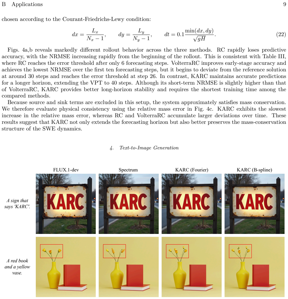
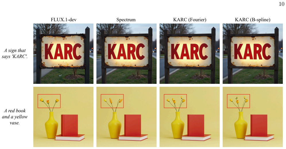
- Can be integrated with generative diffusion models for facilitating text-to-image generation.
- Establishes a principled bridge between reservoir computing and Kolmogorov-Arnold networks.
- Yields a unified framework for efficient dynamical forecasting and generative modeling.
Where Pith is reading between the lines
- The closed-form training could simplify scaling to longer time horizons compared with methods that require recurrence or feature explosion.
- Integration with diffusion models may support hybrid models that enforce physical constraints in generative tasks beyond images.
- The approach might reduce hyperparameter sensitivity that affects conventional reservoir computing.
- Application to real-world time series from climate or fluid dynamics could test whether the basis expansions generalize beyond the reported PDE benchmarks.
Load-bearing premise
The selected basis-function expansions will capture long-range dependencies in the target dynamical systems without recurrence or rapid feature growth.
What would settle it
Showing that KARC fails to outperform standard reservoir computing or next-generation reservoir computing on PDE forecasting tasks at comparable computational cost would falsify the central performance claim.
Figures




read the original abstract
Reservoir computing offers a lightweight framework for forecasting dynamical systems but may struggle to capture long-range dependencies due to limited representational capacity. Conventional reservoir computing recurrently uses fixed reservoirs with hyperparameter sensitivity, while the next generation reservoir computing removes recurrence at the cost of rapidly growing feature dimensions. Here, we develop Kolmogorov-Arnold Reservoir Computing (KARC), which replaces reservoirs with explicit basis-function expansions inspired by the Kolmogorov-Arnold representation theorem. We rigorously show that KARC is a lightweight design of Kolmogorov-Arnold networks (KANs), preserving the potential expressive capacity of KANs while admitting efficient closed-form training of reservoir computing. At comparable cost, KARC outperforms existing reservoir computing methods on challenging benchmarks including partial differential equations. It can also be integrated with generative diffusion models for facilitating text-to-image generation. This work thus establishes a principled bridge between reservoir computing and KANs, yielding a unified framework for efficient dynamical forecasting and generative modeling.
Editorial analysis
A structured set of objections, weighed in public.
Referee Report
Summary. The manuscript introduces Kolmogorov-Arnold Reservoir Computing (KARC), which replaces recurrent reservoirs with explicit univariate basis-function expansions drawn from the Kolmogorov-Arnold representation theorem. It claims to rigorously establish that KARC is a lightweight realization of Kolmogorov-Arnold networks (KANs) that retains their expressive capacity while permitting closed-form linear training, and that it outperforms standard and next-generation reservoir computing on PDE forecasting benchmarks at comparable cost; an additional integration with diffusion models for text-to-image generation is mentioned.
Significance. If the central claims hold, the work supplies a principled bridge between reservoir computing and KANs, yielding a framework that avoids both recurrence and rapid feature-dimension growth while preserving the potential for high expressivity in dynamical forecasting and generative tasks.
major comments (2)
- [Abstract] The central claim that fixed explicit basis expansions capture long-range dependencies in PDEs without recurrence or dimension growth is load-bearing for the outperformance assertion, yet the manuscript supplies no scaling analysis versus prediction horizon, versus basis size, or versus system stiffness to test this assumption (see skeptic note on the weakest assumption).
- [Abstract] The abstract asserts a 'rigorous' proof that KARC is a lightweight KAN design admitting closed-form training, but provides neither the relevant equations, the explicit form of the basis expansions, nor the regularization procedure; without these the soundness of the closed-form claim cannot be assessed.
minor comments (2)
- Dataset details, error bars, and hyperparameter selection protocol for the PDE benchmarks are absent from the abstract and should be supplied with the experimental results.
- The integration with generative diffusion models is stated without any description of how the KARC component is inserted or evaluated; this section requires at least a schematic and quantitative results.
Simulated Author's Rebuttal
We thank the referee for their constructive comments, which help improve the clarity and rigor of our work. We address each major comment in detail below.
read point-by-point responses
-
Referee: [Abstract] The central claim that fixed explicit basis expansions capture long-range dependencies in PDEs without recurrence or dimension growth is load-bearing for the outperformance assertion, yet the manuscript supplies no scaling analysis versus prediction horizon, versus basis size, or versus system stiffness to test this assumption (see skeptic note on the weakest assumption).
Authors: We agree that explicit scaling analyses would strengthen the manuscript. Our current experiments demonstrate outperformance on PDE benchmarks with different prediction horizons and system types, but we did not include dedicated scaling studies. In the revised version, we will add scaling plots versus prediction horizon, basis size, and stiffness parameters to directly test the assumption. revision: yes
-
Referee: [Abstract] The abstract asserts a 'rigorous' proof that KARC is a lightweight KAN design admitting closed-form training, but provides neither the relevant equations, the explicit form of the basis expansions, nor the regularization procedure; without these the soundness of the closed-form claim cannot be assessed.
Authors: The abstract is a high-level summary. The rigorous proof that KARC is a lightweight KAN, the explicit univariate basis expansions (based on the Kolmogorov-Arnold theorem), and the closed-form training via regularized linear regression are provided in detail in Sections 2-4 of the manuscript, including the relevant equations for the basis functions and the training procedure. To address the concern, we will revise the abstract to include a brief reference to these sections and key elements of the formulation. revision: yes
Circularity Check
No circularity; derivation is self-contained via explicit basis replacement and linear readout.
full rationale
The paper defines KARC by replacing the reservoir with fixed univariate basis expansions drawn from the Kolmogorov-Arnold theorem, then shows that the resulting model admits a closed-form linear solution for the readout weights exactly as in standard reservoir computing. This reduction follows directly from the linearity of the final layer with respect to the chosen basis coefficients and does not rely on fitting any target quantity to itself or on self-citation chains that presuppose the result. The expressive-capacity claim is an existence statement inherited from the representation theorem rather than a fitted prediction, and no step renames an empirical pattern or imports a uniqueness result from the authors' prior work as an external fact. The derivation therefore remains independent of its own outputs.
Axiom & Free-Parameter Ledger
axioms (1)
- standard math Kolmogorov-Arnold representation theorem guarantees that the required multivariate functions can be expressed as finite sums of univariate functions.
Reference graph
Works this paper leans on
- [1]
-
[2]
N. Kovachki, Z. Li, B. Liu, K. Azizzadenesheli, K. Bhattacharya, A. Stuart, and A. Anandkumar, Neural operator: Learning maps between function spaces with applications to PDEs, J. Mach. Learn. Res. 24, 1 (2023)
work page 2023
-
[3]
Empirical Evaluation of Gated Recurrent Neural Networks on Sequence Modeling
J. Chung, C. Gulcehre, K. Cho, and Y. Bengio, Empirical evaluation of gated recurrent neural networks on sequence modeling, arXiv preprint arXiv:1412.3555 (2014)
work page internal anchor Pith review Pith/arXiv arXiv 2014
-
[4]
A. Vaswani, N. Shazeer, N. Parmar, J. Uszkoreit, L. Jones, A. N. Gomez, Ł. Kaiser, and I. Polosukhin, Attention is all you need, in Advances in Neural Information Processing Systems , Vol. 30 (2017) pp. 5998–6008
work page 2017
-
[5]
Z. Li, N. B. Kovachki, K. Azizzadenesheli, B. liu, K. Bhattacharya, A. Stuart, and A. Anandkumar, Fourier neural operator for parametric partial differential equations, in Int. Conf. Learn. Represent. (2021)
work page 2021
-
[6]
T. Wang and C. Wang, Latent neural operator for solving forward and inverse PDE problems, in Adv. Neural Inf. Process. Syst., Vol. 37 (2024)
work page 2024
-
[7]
L. Lu, P. Jin, G. Pang, Z. Zhang, and G. E. Karniadakis, Learning nonlinear operators via DeepONet based on the universal approximation theorem of operators, Nat. Mach. Intell. 3, 218 (2021)
work page 2021
-
[8]
S. Goswami, A. Bora, Y. Yu, and G. E. Karniadakis, Physics-informed deep neural operator networks, in Machine Learning in Modeling and Simulation: Methods and Applications , Computational Methods in Engineering & the Sciences, edited by T. Rabczuk and K.-J. Bathe (Springer, 2023) pp. 219–254
work page 2023
-
[9]
N. B. Kovachki, S. Lanthaler, and A. M. Stuart, Operator learning: Algorithms and analysis, in Numerical Analysis Meets Machine Learning , Handb. Numer. Anal., Vol. 25 (Elsevier, 2024) pp. 419–467
work page 2024
-
[10]
S. Liu, Y. Yu, T. Zhang, H. Liu, X. Liu, and D. Meng, Architectures, variants, and performance of neural operators: A comparative review, Neurocomputing 648, 130518 (2025)
work page 2025
-
[11]
K. Benidis, S. S. Rangapuram, V. Flunkert, Y. Wang, D. Maddix, C. Turkmen, J. Gasthaus, M. Bohlke-Schneider, D. Salinas, L. Stella, et al. , Deep learning for time series forecasting: Tutorial and literature survey, ACM Comput. Surv. 55, 1 (2022)
work page 2022
- [13]
-
[15]
N. Lin, S. Wang, Y. Li, B. Wang, S. Shi, Y. He, W. Zhang, Y. Yu, Y. Zhang, X. Zhang, et al. , Resistive memory-based zero-shot liquid state machine for multimodal event data learning, Nat. Comput. Sci. 5, 37 (2025)
work page 2025
-
[16]
R. S. Zimmermann and U. Parlitz, Observing spatio-temporal dynamics of excitable media using reservoir computing, Chaos 28, 043118 (2018)
work page 2018
-
[17]
Y. Xiong and H. Zhao, Chaotic time series prediction based on long short-term memory neural networks, Sci. China Phy. Mech. Astron. 49, 120501 (2019)
work page 2019
-
[18]
H. Fan, J. Jiang, C. Zhang, X. Wang, and Y.-C. Lai, Long-term prediction of chaotic systems with machine learning, Phys. Rev. Res. 2, 012080 (2020)
work page 2020
-
[19]
M. Rafayelyan, J. Dong, Y. Tan, F. Krzakala, and S. Gigan, Large-scale optical reservoir computing for spatiotemporal chaotic systems prediction, Phys. Rev. X 10, 041037 (2020)
work page 2020
-
[20]
Z. Lin, Z. Lu, Z. Di, and Y. Tang, Learning noise-induced transitions by multi-scaling reservoir computing, Nat. Commun. 15, 6584 (2024)
work page 2024
-
[21]
H. Tan, L. Shi, S. Wang, and S.-X. Qu, Improving model-free prediction of chaotic dynamics by purifying the incomplete input, AIP Adv. 14 (2024)
work page 2024
-
[22]
X. Li, Q. Zhu, C. Zhao, X. Duan, B. Zhao, X. Zhang, H. Ma, J. Sun, and W. Lin, Higher-order granger reservoir D Error Bound of KARC for Fading Memory Dynamical Systems 22 computing: simultaneously achieving scalable complex structures inference and accurate dynamics prediction, Nat. Commun. 15, 2506 (2024)
work page 2024
-
[23]
X. Han, Z. Qi, V. Kundrat, H. Li, Z. Li, X. Guo, P. Mao, W. Zheng, S. Hou, R. Liu, et al. , Very-large-scale mimetic optogenetic synapses for physical reservoir computing, Nat. Commun. 17, 1514 (2026)
work page 2026
- [24]
-
[25]
L. Grigoryeva and J.-P. Ortega, Universal discrete-time reservoir computers with stochastic inputs and linear readouts using non-homogeneous state-affine systems, J. Mach. Learn. Res. 19, 1 (2018)
work page 2018
-
[26]
L. Grigoryeva and J.-P. Ortega, Echo state networks are universal, Neural Netw. 108, 495 (2018)
work page 2018
-
[27]
L. Gonon and J.-P. Ortega, Reservoir computing universality with stochastic inputs, IEEE Trans. Neural Netw. Learn. Syst. 31, 100 (2019)
work page 2019
-
[28]
A. Hart, J. Hook, and J. Dawes, Embedding and approximation theorems for echo state networks, Neural Netw. 128, 234 (2020)
work page 2020
-
[29]
L. Gonon and J.-P. Ortega, Fading memory echo state networks are universal, Neural Netw. 138, 10 (2021)
work page 2021
-
[30]
L. A. Thiede and U. Parlitz, Gradient based hyperparameter optimization in echo state networks, Neural Netw. 115, 23 (2019)
work page 2019
- [31]
-
[32]
M. Yan, C. Huang, P. Bienstman, P. Tino, W. Lin, and J. Sun, Emerging opportunities and challenges for the future of reservoir computing, Nat. Commun. 15, 2056 (2024)
work page 2056
-
[33]
M. Lukoševičius and H. Jaeger, Reservoir computing approaches to recurrent neural network training, Comput. Sci. Rev. 3, 127 (2009)
work page 2009
-
[34]
E. Martin and C. Cundy, Parallelizing linear recurrent neural nets over sequence length, in Int. Conf. Learn. Represent. (2018)
work page 2018
-
[35]
D. J. Gauthier, E. Bollt, A. Griffith, and W. A. S. Barbosa, Next generation reservoir computing, Nat. Commun. 12, 5564 (2021)
work page 2021
-
[37]
L. Grigoryeva, H. L. J. Ting, and J.-P. Ortega, Infinite-dimensional next-generation reservoir computing, Phys. Rev. E 111, 035305 (2025)
work page 2025
-
[38]
R. Cestnik and E. A. Martens, Next-generation reservoir computing for dynamical inference, Chaos 36, 013115 (2026)
work page 2026
-
[39]
A. N. Kolmogorov, On the representation of continuous functions of many variables by superposition of continuous functions of one variable and addition, Dokl. Akad. Nauk SSSR 114, 953 (1957)
work page 1957
-
[40]
Z. Liu, Y. Wang, S. Vaidya, F. Ruehle, J. Halverson, M. Soljačić, T. Y. Hou, and M. Tegmark, KAN: Kolmogorov-arnold networks, in Proceedings of the International Conference on Learning Representations (2025)
work page 2025
-
[41]
Z. Liu, M. Tegmark, P. Ma, W. Matusik, and Y. Wang, Kolmogorov-arnold networks meet science, Phys. Rev. X 15, 041051 (2025)
work page 2025
-
[42]
MesaNet: Sequence Modeling by Locally Optimal Test-Time Training
J. von Oswald, N. Scherrer, S. Kobayashi, L. Versari, S. Yang, M. Schlegel, K. Maile, Y. Schimpf, O. Sieberling, A. Meulemans, et al. , Mesanet: Sequence modeling by locally optimal test-time training, arXiv:2506.05233 (2025)
work page internal anchor Pith review Pith/arXiv arXiv 2025
-
[43]
J. Han, J. Shi, P. Li, H. Ye, Q. Guo, and S. Ermon, Adaptive spectral feature forecasting for diffusion sampling acceleration, in Proceedings of the IEEE/CVF Conference on Computer Vision and Pattern Recognition (2026) pp. 43320–43330
work page 2026
- [44]
-
[45]
G. K. Vallis, Atmospheric and Oceanic Fluid Dynamics: Fundamentals and Large-Scale Circulation , 2nd ed. (Cambridge University Press, 2017)
work page 2017
-
[47]
G. Li, L. Huang, and Y. Lei, Reservoir computing meeting kolmogorov-arnold networks: prediction of high-dimensional chaotic systems, Chaos 35, 103120 (2025)
work page 2025
-
[48]
Z. Lin, J. Kurths, and Y. Tang, Multi-scaling reservoir computing learns noise-induced transitions with Lévy noise, Chaos 35, 073132 (2025)
work page 2025
- [49]
-
[50]
Z. Li, H. Zheng, N. Kovachki, D. Jin, H. Chen, B. Liu, K. Azizzadenesheli, and A. Anandkumar, Physics-informed neural operator for learning partial differential equations, ACM/IMS J. Data Sci. 1, 1 (2024) . Supplementary Information: Kolmogorov-Arnold Reservoir Computing Juntian Huang, 1 Jürgen Kurths, 2, 3, 4 and Ying Tang 1, 5, 6, 7, ∗ 1Institute of Fun...
work page 2024
-
[51]
D. J. Gauthier, E. Bollt, A. Griffith, and W. A. S. Barbosa, Next generation reservoir computing, Nat. Commun. 12, 5564 (2021)
work page 2021
-
[52]
L. Grigoryeva, H. L. J. Ting, and J.-P. Ortega, Infinite-dimensional next-generation reservoir computing, Phys. Rev. E 111, 035305 (2025)
work page 2025
-
[53]
H. Jaeger, The “echo state” approach to analysing and training recurrent neural networks–with an erratum note , GMD Technical Report 148 (German National Research Center for Information Technology, Bonn, Germany, 2001)
work page 2001
- [54]
-
[55]
E. Bollt, On explaining the surprising success of reservoir computing forecaster of chaos? the universal machine learning dynamical system with contrast to var and dmd, Chaos 31, 013108 (2021)
work page 2021
-
[56]
Black Forest Labs, FLUX, https://github.com/black-forest-labs/flux (2024), gitHub repository
work page 2024
-
[57]
J. Han, J. Shi, P. Li, H. Ye, Q. Guo, and S. Ermon, Adaptive spectral feature forecasting for diffusion sampling accelera- tion, in Proceedings of the IEEE/CVF Conference on Computer Vision and Pattern Recognition (2026) pp. 43320–43330
work page 2026
-
[58]
Z. Li, N. B. Kovachki, K. Azizzadenesheli, B. liu, K. Bhattacharya, A. Stuart, and A. Anandkumar, Fourier neural operator for parametric partial differential equations, in Int. Conf. Learn. Represent. (2021)
work page 2021
discussion (0)
Sign in with ORCID, Apple, or X to comment. Anyone can read and Pith papers without signing in.