Pressure reconstruction from error-embedded gradient measurements: a Gaussian-process generalization of Green's function integration
Pith reviewed 2026-06-30 22:08 UTC · model grok-4.3
The pith
Gaussian process regression reconstructs pressure fields from noisy gradient measurements and reduces to Green's function integration when noise vanishes.
A machine-rendered reading of the paper's core claim, the machinery that carries it, and where it could break.
Core claim
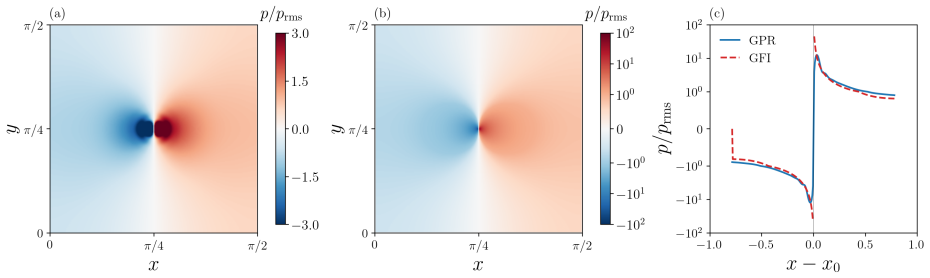
A central theoretical result of the present work is that GFI is the noiseless limit of GPR, which on the unbounded plane reduces to the well-known logarithmic kernel and in three dimensions to the inverse-distance kernel. With an empirical mixture-of-Gaussians kernel fitted directly to the pressure correlation function, GPR performs at least as well as GFI on turbulent flow data while delivering calibrated pointwise posterior uncertainty.
What carries the argument
Gaussian Process Regression (GPR) with an empirical mixture-of-Gaussians kernel, shown to have Green's function integration as its noiseless limit.
If this is right
- GPR supplies tunable denoising and pointwise posterior-variance estimates without explicit boundary conditions.
- On the unbounded plane the method recovers the logarithmic kernel; in three dimensions it recovers the inverse-distance kernel.
- The framework extends to three dimensions via a tensor-product Kronecker solver with near O(N^3 log N) cost.
- A closed-form error lower bound holds on a periodic cube, with the residual gap on finite domains attributed to boundary contamination.
Where Pith is reading between the lines
- The same GPR construction could be applied to other linear inverse problems that recover scalars from noisy gradients, such as temperature or concentration fields.
- Fitting the kernel directly from the noisy observations may allow the method to adapt to non-stationary statistics without separate calibration data.
- The boundary-contamination gap identified on non-periodic domains suggests a possible extension that incorporates known boundary values when they are available.
Load-bearing premise
The pressure field can be treated as a Gaussian process whose covariance is accurately captured by an empirical mixture-of-Gaussians kernel fitted directly to the observed pressure correlation function from the same noisy dataset.
What would settle it
A direct test on held-out turbulence data where the standardized residuals of the GPR posterior fail to satisfy |z| < 2 over at least 95 percent of points, or where GPR reconstruction error exceeds that of Green's function integration under high noise.
Figures




read the original abstract
Reconstructing scalar fields from error-embedded gradient measurements is a fundamental linear inverse problem with broad applications in computational physics. Conventional approaches, such as Poisson-based solvers and the Green's Function Integration (GFI) method, require explicit boundary conditions extracted from the same error-embedded observations. In this study we assess the accuracy of a Gaussian Process Regression (GPR) framework for reconstructing pressure fields in turbulent flows from error-embedded pressure-gradient data derived from kinematic measurements. The probabilistic nature of GPR inherently provides tunable denoising, eliminates the need for boundary conditions, and produces a pointwise posterior-variance error estimate. A central theoretical result of the present work is that GFI is the noiseless limit of GPR, which on the unbounded plane reduces to the well-known logarithmic kernel and in three dimensions to the inverse-distance kernel. The framework is validated on two-dimensional slices and three-dimensional subdomains of a forced homogeneous isotropic turbulence from the Johns Hopkins Turbulence Database. With an empirical mixture-of-Gaussians (MoG-$3$) kernel fitted directly to the pressure correlation function, GPR performs at least as well as GFI. In situations with under-resolved data or high noise, GPR outperforms GFI, while delivering a calibrated pointwise posterior uncertainty whose standardized residuals satisfy $|z|<2$ over $95\%$ of grid points. The framework extends to three dimensions through a tensor-product Kronecker solver coupled to conjugate gradients with close to $\mathcal{O}(N^3\log N)$ cost. A closed-form error lower bound on a periodic cube is derived for the GPR operator, with the residual gap attributable to boundary contamination on non-periodic finite domains.
Editorial analysis
A structured set of objections, weighed in public.
Referee Report
Summary. The manuscript proposes a Gaussian Process Regression (GPR) framework for reconstructing pressure fields from error-embedded gradient measurements in turbulent flows. It claims that Green's Function Integration (GFI) is the noiseless limit of GPR, reducing to the logarithmic kernel on the unbounded plane (2D) and the inverse-distance kernel (3D). Validation on 2D slices and 3D subdomains from the Johns Hopkins Turbulence Database uses an empirical MoG-3 kernel fitted to the pressure correlation function; GPR matches or exceeds GFI performance (especially under noise) while providing calibrated posterior uncertainty with |z|<2 on 95% of points. A closed-form error lower bound is derived for periodic domains, and a Kronecker-based 3D solver is presented.
Significance. If the central equivalence holds and the uncertainty calibration generalizes, the work offers a boundary-condition-free probabilistic alternative to Poisson solvers and GFI with built-in error estimates, which would be useful for inverse problems in fluid dynamics. Strengths include the efficient 3D implementation and the closed-form error bound on periodic cubes. The data-driven kernel fitting, however, limits claims of broad superiority.
major comments (2)
- [Abstract] Abstract (central theoretical result): The claim that GFI is the noiseless limit of GPR reducing to the logarithmic kernel (2D) and inverse-distance kernel (3D) is load-bearing but requires explicit handling. These kernels are only conditionally positive definite with spectral density ~1/|k|^2, non-integrable at k=0, and yield formally infinite pointwise variance; standard GPR posterior formulas assume a proper positive-definite kernel with finite K(0). The manuscript does not specify modifications (e.g., polynomial null space, increments, or fixed-mean constraints) needed to make the noiseless limit well-posed within the GPR framework used elsewhere.
- [Abstract] Validation paragraph (abstract): The MoG-3 kernel (3 weights, 3 means, 3 variances) is fitted directly to the pressure correlation function extracted from the same JHTDB slices used for validation. This makes the reported performance advantage of GPR over GFI in under-resolved or high-noise regimes dependent on a data-driven covariance that is not independent of the test data, undermining generalizability claims.
Simulated Author's Rebuttal
We thank the referee for their careful reading and valuable comments on our manuscript. We address the major comments point by point below, and have revised the manuscript accordingly where appropriate.
read point-by-point responses
-
Referee: [Abstract] Abstract (central theoretical result): The claim that GFI is the noiseless limit of GPR reducing to the logarithmic kernel (2D) and inverse-distance kernel (3D) is load-bearing but requires explicit handling. These kernels are only conditionally positive definite with spectral density ~1/|k|^2, non-integrable at k=0, and yield formally infinite pointwise variance; standard GPR posterior formulas assume a proper positive-definite kernel with finite K(0). The manuscript does not specify modifications (e.g., polynomial null space, increments, or fixed-mean constraints) needed to make the noiseless limit well-posed within the GPR framework used elsewhere.
Authors: We appreciate the referee pointing out this subtlety in the theoretical foundation. The central claim is that as the noise variance approaches zero, the GPR posterior mean converges to the GFI solution obtained via the Green's function corresponding to those kernels. In the revised manuscript, we will explicitly state that the logarithmic and inverse-distance kernels are employed in the sense of generalized functions or with a suitable null-space handling (e.g., by subtracting the mean or using increments) to address their conditional positive definiteness. We will add a brief discussion in the methods section clarifying how the noiseless limit is taken within the GPR framework, ensuring consistency with standard GPR assumptions for finite noise levels. revision: yes
-
Referee: [Abstract] Validation paragraph (abstract): The MoG-3 kernel (3 weights, 3 means, 3 variances) is fitted directly to the pressure correlation function extracted from the same JHTDB slices used for validation. This makes the reported performance advantage of GPR over GFI in under-resolved or high-noise regimes dependent on a data-driven covariance that is not independent of the test data, undermining generalizability claims.
Authors: The referee is correct that fitting the kernel to the correlation function from the validation dataset introduces a dependence that affects the interpretation of generalizability. This setup demonstrates the potential of GPR when the covariance structure is known from the flow statistics, as is common in turbulence studies. However, to strengthen the manuscript, we will revise the abstract and discussion to qualify that the performance comparison is for this specific dataset with kernel fitted to its statistics, and note that for new flows the kernel would need to be determined independently (e.g., from separate simulations or theory). We do not claim broad superiority beyond the tested conditions. revision: partial
Circularity Check
No significant circularity in the derivation chain
full rationale
The central theoretical result that GFI is the noiseless limit of GPR (reducing to the logarithmic kernel in 2D and inverse-distance kernel in 3D) is presented as a derived mathematical equivalence independent of data. The empirical MoG-3 kernel is fitted to the pressure correlation function as a methodological choice for validation on the JHU turbulence database, but this does not reduce the theoretical claim or performance statements to the inputs by construction. No self-citations, self-definitional steps, or fitted parameters renamed as predictions are quoted in the provided text that would force the result. The derivation chain is self-contained against the stated assumptions.
Axiom & Free-Parameter Ledger
free parameters (1)
- MoG-3 kernel parameters (3 weights, 3 means, 3 variances)
axioms (2)
- domain assumption The pressure field is a realization of a Gaussian process with stationary covariance given by the chosen kernel.
- domain assumption The noise in the gradient measurements is additive, zero-mean, and uncorrelated with the signal.
Reference graph
Works this paper leans on
-
[1]
X. Liu, J. Katz, Measurements of pressure distribution by integrating the material acceleration, in: Cav03-GS-14-001, Fifth international symposium on cavitation (CAV2003), Osaka, Japan, 2003, pp. 1–4
2003
-
[2]
X. Liu, J. Katz, Instantaneous pressure and material acceleration measurements using a four-exposure piv system, Experiments in fluids 41 (2006) 227–240
2006
-
[3]
D. A. Buchta, J. B. Freund, The near-field pressure radiated by planar high-speed free-shear-flow turbulence, Journal of Fluid Mechanics 832 (2017) 383–408
2017
-
[4]
S. F. Wu, Methods for reconstructing acoustic quantities based on acoustic pressure measurements, The Journal of the Acoustical Society of America 124 (2008) 2680–2697
2008
-
[5]
R. A. Gramann, D. S. Dolling, Detection of turbulent boundary-layer separation using fluctuating wall pressure signals, AIAA journal 28 (1990) 1052–1056
1990
-
[6]
Cerretelli, K
C. Cerretelli, K. Kirtley, Boundary layer separation control with fluidic oscillators (2009)
2009
-
[7]
Yeung, D
P. Yeung, D. Donzis, K. Sreenivasan, Dissipation, enstrophy and pressure statistics in turbulence simulations at high reynolds numbers, Journal of Fluid Mechanics 700 (2012) 5–15
2012
-
[8]
M. A. Abassi, Q. Wang, X. Liu, Adjoint-based data assimilation in a subdomain using omnidirectional- integration-enabled pressure dirichlet boundary conditions, Physics of Fluids 37 (2025)
2025
-
[9]
T. A. Zaki, Turbulence from an observer perspective, Annual Review of Fluid Mechanics 57 (2025) 311–334
2025
-
[10]
X. Liu, J. R. Moreto, S. Siddle-Mitchell, Instantaneous pressure reconstruction from measured pressure gradient using rotating parallel ray method, in: 54th AIAA Aerospace Sciences Meeting, 2016, p. 1049
2016
-
[11]
X. Liu, J. Katz, Pressure–rate-of-strain, pressure diffusion, and velocity–pressure-gradient tensor mea- surements in a cavity flow, AIAA Journal 56 (2018) 3897–3914. 23
2018
-
[12]
J. R. Moreto, W. J. Reeder, R. Budwig, D. Tonina, X. Liu, Experimentally mapping water surface elevation, velocity, and pressure fields of an open channel flow around a stalk, Geophysical Research Letters 49 (2022) e2021GL096835
2022
-
[13]
X. Liu, J. R. Moreto, Error propagation from the piv-based pressure gradient to the integrated pressure by the omnidirectional integration method, Measurement Science and Technology 31 (2020) 055301
2020
-
[14]
Q. Wang, X. Liu, Green’s function integral method for pressure reconstruction from measured pressure gradient and the interpretation of omnidirectional integration, Physics of Fluids 35 (2023)
2023
-
[15]
Zigunov, J
F. Zigunov, J. J. Charonko, One-shot omnidirectional pressure integration through matrix inversion, Measurement Science and Technology 35 (2024) 125301
2024
-
[16]
C. E. Rasmussen, C. K. I. Williams, Gaussian Processes for Machine Learning, MIT Press, 2006
2006
-
[17]
Schulz, M
E. Schulz, M. Speekenbrink, A. Krause, A tutorial on gaussian process regression: Modelling, exploring, and exploiting functions, Journal of Mathematical Psychology 85 (2018) 1–16
2018
-
[18]
V. Mons, Q. Wang, T. A. Zaki, Kriging-enhanced ensemble variational data assimilation for scalar- source identification in turbulent environments, Journal of Computational Physics 398 (2019) 108856
2019
-
[19]
Z. You, Q. Wang, X. Liu, Pressure reconstruction from the measured pressure gradient using gaussian process regression, in: AIAA SCITECH 2023 Forum, 2023, p. 0414
2023
-
[20]
Solak, R
E. Solak, R. Murray-Smith, W. E. Leithead, D. J. Leith, C. E. Rasmussen, Derivative observations in Gaussian process models of dynamic systems, in: Advances in Neural Information Processing Systems 15, 2003, pp. 1057–1064
2003
-
[21]
Wahba, Spline Models for Observational Data, volume 59 ofCBMS-NSF Regional Conference Series in Applied Mathematics, SIAM, 1990
G. Wahba, Spline Models for Observational Data, volume 59 ofCBMS-NSF Regional Conference Series in Applied Mathematics, SIAM, 1990
1990
-
[22]
Hastie, R
T. Hastie, R. Tibshirani, J. Friedman, et al., The elements of statistical learning, 2009
2009
-
[23]
Kimeldorf, G
G. Kimeldorf, G. Wahba, Some results on Tchebycheffian spline functions, Journal of Mathematical Analysis and Applications 33 (1971) 82–95
1971
-
[24]
Gaussian Processes and Kernel Methods: A Review on Connections and Equivalences
M. Kanagawa, P. Hennig, D. Sejdinovic, B. K. Sriperumbudur, Gaussian processes and kernel methods: A review on connections and equivalences, arXiv preprint arXiv:1807.02582 (2018)
work page internal anchor Pith review Pith/arXiv arXiv 2018
-
[25]
A. J. Smola, B. Schölkopf, Learning with kernels, volume 4, GMD-Forschungszentrum Informationstech- nik Berlin, Germany, 1998
1998
-
[26]
Graepel, Solving noisy linear operator equations by gaussian processes: Application to ordinary and partial differential equations, in: ICML, volume 3, 2003, pp
T. Graepel, Solving noisy linear operator equations by gaussian processes: Application to ordinary and partial differential equations, in: ICML, volume 3, 2003, pp. 234–241
2003
-
[27]
Cockayne, C
J. Cockayne, C. Oates, T. Sullivan, M. Girolami, Probabilistic numerical methods for pde-constrained bayesian inverse problems, in: AIP Conference Proceedings, volume 1853, AIP Publishing LLC, 2017, p. 060001
2017
-
[28]
Raissi, P
M. Raissi, P. Perdikaris, G. E. Karniadakis, Machine learning of linear differential equations using gaussian processes, Journal of Computational Physics 348 (2017) 683–693
2017
-
[29]
L. P. Swiler, M. Gulian, A. L. Frankel, C. Safta, J. D. Jakeman, A survey of constrained gaussian process regression: Approaches and implementation challenges, Journal of Machine Learning for Modeling and Computing 1 (2020)
2020
-
[30]
A. P. Valentine, M. Sambridge, Gaussian process models—i. a framework for probabilistic continuous inverse theory, Geophysical Journal International 220 (2020) 1632–1647. 24
2020
-
[31]
Dalton, A
D. Dalton, A. Lazarus, H. Gao, D. Husmeier, Boundary constrained gaussian processes for robust physics-informed machine learning of linear partial differential equations, Journal of Machine Learning Research 25 (2024) 1–61
2024
- [32]
-
[33]
X. Li, M. Lange-Hegermann, B. Raitˇ a, Gaussian process regression for inverse problems in linear pdes, IFAC-PapersOnLine 59 (2025) 196–201
2025
-
[34]
E. J. Parish, K. Duraisamy, A paradigm for data-driven predictive modeling using field inversion and machine learning, Journal of computational physics 305 (2016) 758–774
2016
-
[35]
M. Wang, Q. Wang, T. A. Zaki, Discrete adjoint of fractional-step incompressible navier-stokes solver in curvilinear coordinates and application to data assimilation, Journal of Computational Physics 396 (2019) 427–450
2019
-
[36]
M. R. Hestenes, E. Stiefel, Methods of conjugate gradients for solving linear systems, Journal of Research of the National Bureau of Standards 49 (1952) 409–436. doi:10.6028/jres.049.044
-
[37]
Y. Li, E. Perlman, M. Wan, Y. Yang, C. Meneveau, R. Burns, S. Chen, A. Szalay, G. Eyink, A public turbulence database cluster and applications to study lagrangian evolution of velocity increments in turbulence, Journal of Turbulence (2008) N31
2008
-
[38]
Perlman, R
E. Perlman, R. Burns, Y. Li, C. Meneveau, Data exploration of turbulence simulations using a database cluster, in: Proceedings of the 2007 ACM/IEEE Conference on Supercomputing, 2007, pp. 1–11
2007
-
[39]
Aronszajn, Theory of reproducing kernels, Transactions of the American Mathematical Society 68 (1950) 337–404
N. Aronszajn, Theory of reproducing kernels, Transactions of the American Mathematical Society 68 (1950) 337–404
1950
-
[40]
H. Taha, C. Gonzalez, M. Shorbagy, A minimization principle for incompressible fluid mechanics, Physics of Fluids 35 (2023)
2023
-
[41]
Strang, A proposal for Toeplitz matrix calculations, Studies in Applied Mathematics 74 (1986) 171–176
G. Strang, A proposal for Toeplitz matrix calculations, Studies in Applied Mathematics 74 (1986) 171–176
1986
-
[42]
Greengard, J
L. Greengard, J. Strain, The fast Gauss transform, SIAM Journal on Scientific and Statistical Com- puting 12 (1991) 79–94
1991
-
[43]
J. Wang, C. Zhang, J. Katz, Gpu-based, parallel-line, omni-directional integration of measured pressure gradient field to obtain the 3d pressure distribution, Experiments in Fluids 60 (2019) 58
2019
-
[44]
Bochner, Harmonic analysis and the theory of probability, Courier Corporation, 2005
S. Bochner, Harmonic analysis and the theory of probability, Courier Corporation, 2005
2005
-
[45]
M. L. Stein, Interpolation of spatial data: some theory for kriging, Springer Science & Business Media, 1999
1999
-
[46]
Q. Wang, M. Wang, T. A. Zaki, What is observable from wall data in turbulent channel flow?, Journal of Fluid Mechanics 941 (2022) A48. doi:10.1017/jfm.2022.295
-
[47]
Q. Wang, Y. Hasegawa, T. A. Zaki, Spatial reconstruction of steady scalar sources from remote mea- surements in turbulent flow, Journal of Fluid Mechanics 870 (2019) 316–352
2019
-
[48]
E. C. Howell, J. D. Hanson, Development of a non-parametric gaussian process model in the three- dimensional equilibrium reconstruction code v3fit, Journal of Plasma Physics 86 (2020) 905860102. doi:10.1017/S0022377819000813
-
[49]
Y. Yang, Y. Xue, W. Zhao, S. Yao, C. Li, C. Wu, Fast flow field prediction of three-dimensional hypersonic vehicles using an improved gaussian process regression algorithm, Physics of Fluids 36 (2024). 25
2024
discussion (0)
Sign in with ORCID, Apple, or X to comment. Anyone can read and Pith papers without signing in.