Learning to Emulate Chaos: Adversarial Optimal Transport Regularization
Pith reviewed 2026-07-05 01:30 UTC · model glm-5.2
The pith
Adversarial Optimal Transport Trains Chaos Emulators from One Noisy Trajectory
A machine-rendered reading of the paper's core claim, the machinery that carries it, and where it could break.
Core claim
The central mechanism is an adversarial min-max objective over an emulator g and a summary map f. The emulator minimizes a combined loss of one-step MSE and a Wasserstein distance between the pushforward measures f#μ (true data) and f#ĝ (emulator output), while the summary map maximizes that same Wasserstein distance. This forces f to find the statistics where the emulator most badly fails, and forces g to fix exactly those failures. The theoretical analysis establishes a clean separation: MSE captures short-horizon trajectory fidelity but diverges exponentially under noise at long horizons due to chaotic amplification through the Jacobian, while the Wasserstein term captures long-horizon统计f
What carries the argument
The adversarial optimal transport objective in Eq. (4), instantiated as either a WGAN-style dual (Eq. 6) or a Sinkhorn divergence (Eq. 8). The noise robustness theorem (Theorem 5.14) relies on the assumption that the emulator is exponentially mixing in Wp, meaning the emulator's induced dynamics forget initial condition perturbations at a geometric rate, so the Wasserstein distance between the true invariant measure and the emulator's noisy rollout measure converges to a finite limit independent of the initial condition noise.
If this is right
- If the approach generalizes beyond the tested benchmarks, it could enable data-efficient surrogate models for climate simulation, turbulence modeling, and plasma physics that are trained from a single observational run rather than requiring large multi-scenario datasets.
- The adversarial summary learning mechanism could be applied to other distribution-matching problems where the choice of test statistics is non-obvious, such as simulation-based inference or generative model evaluation in scientific domains.
- The theoretical separation between trajectory-level losses (which diverge under chaos) and distributional losses (which remain bounded) provides a principled basis for designing training curricula that shift weight from MSE to OT as the rollout horizon exceeds the system's mixing time.
- The ability to recover accurate Lyapunov exponents (Table 3) suggests the learned emulators preserve not just static statistics but dynamical invariants, which could make them useful for bifurcation analysis and stability studies of the underlying physical systems.
Where Pith is reading between the lines
- The exponential mixing assumption on the learned emulator (Definition 5.12) is the load-bearing condition for noise robustness. If one could establish that the adversarial training procedure itself encourages or guarantees mixing — for instance, because matching the invariant measure under a Lipschitz summary map constrains the emulator's spectral properties — this would close the gap between theo
- The displacement covariance result (Proposition A.1) suggests that the learned linear summary maps are implicitly performing a form of principal component analysis on the optimal transport displacement field, which connects the adversarial summary learning to spectral analysis of the transport plan.
- The framework could potentially be extended to non-ergodic or transient systems by replacing the global invariant measure with a time-windowed empirical measure, though the theoretical guarantees on noise forgetting would need to be reformulated for non-stationary dynamics.
- The observation that Sinkhorn training requires early stopping to prevent degenerate collapse of the summary map (Appendix C.1) suggests that the entropic regularization parameter and the adversarial training dynamics interact in ways that are not fully captured by the population-level theory, pointing to a need for finite-sample analysis of the min-max game.
Load-bearing premise
The noise robustness theorem assumes the trained emulator is exponentially mixing — meaning its dynamics forget initial perturbations at a geometric rate — but there is no proof that the training procedure produces an emulator with this property; it is empirically observed on the tested benchmarks but could fail for unstable or poorly trained models. The paper also acknowledges that the analysis does not guarantee the existence of a saddle point for the full min-max objective
What would settle it
If the exponential mixing assumption fails for a trained emulator — for example, if the emulator develops a spurious slow manifold or periodic orbit that does not forget initial perturbations — then the Wasserstein noise forgetting bound (Theorem 5.14) would not hold and the OT regularizer could become noise-dominated just like MSE. Empirically, this would manifest as the OT-regularized emulator degrading at long rollout horizons under noise, similar to the MSE-only baseline.
Figures






read the original abstract
Chaos arises in many complex dynamical systems, from weather to power grids, but is difficult to accurately model with data-driven methods such as machine learning emulators. While emulators are promising tools for accelerating simulations and solving inverse problems, they still struggle to learn chaotic dynamics, where sensitivity to initial conditions renders exact long-term forecasts infeasible, especially given noisy data. Recent work instead trains emulators to match the statistical properties of chaotic attractors, but these approaches often rely on handcrafted summary statistics or large, diverse multi-environment datasets. In this work, we propose a family of adversarial optimal transport objectives that can jointly learn high-quality summary statistics and a physically consistent emulator from a single noisy trajectory. We theoretically analyze and experimentally validate a Sinkhorn divergence formulation (2-Wasserstein) and a WGAN-style dual formulation (1-Wasserstein) of our approach. Numerical experiments across a variety of chaotic systems, including ones with high-dimensional spatiotemporal chaos, show that emulators trained using our proposed objectives have significantly improved long-term statistical fidelity.
Editorial analysis
A structured set of objections, weighed in public.
Referee Report
Summary. This paper proposes adversarial optimal transport (OT) regularization for training emulators of chaotic dynamical systems. The core idea is to jointly learn an emulator g and a summary map f via a min-max objective (Eq. 4), where the emulator minimizes a combination of MSE and an OT cost between summary distributions of real and generated trajectories, while the summary map maximizes this OT cost to discover informative statistics. Two tractable instantiations are developed: a WGAN-style dual formulation (1-Wasserstein) and a Sinkhorn divergence formulation (2-Wasserstein). Theoretical analysis (Section 5) shows the OT regularizer is bounded by one-step prediction error (Prop. 5.1) and that the Wasserstein objective is robust to initial-condition noise under an exponential mixing assumption on the emulator (Thm. 5.14), unlike MSE which diverges exponentially (Cor. 5.9). Experiments on Lorenz-96, Kuramoto-Sivashinsky, and Kolmogorov flow demonstrate improved long-term statistical fidelity over MSE-only and fixed-statistics OT baselines.
Significance. The paper addresses a practically important problem: training data-driven emulators of chaotic systems from noisy data, where standard trajectory-matching losses are known to fail. The idea of adversarially learning summary statistics via OT, rather than relying on handcrafted features or multi-environment datasets, is a natural and well-motivated contribution that builds on and extends the framework of Jiang et al. (2023). The theoretical results in Section 5.1 are clean: Prop. 5.1 and Cor. 5.2 provide parameter-free bounds linking the summary-space Wasserstein cost to prediction error, and Prop. A.1 gives an exact characterization for the linear summary case. The noise-robustness analysis (Thm. 5.14 vs. Cor. 5.9) provides a clear conceptual distinction between distributional and trajectory-based objectives. The experimental scope across three systems of increasing dimensionality, including a 2D turbulent flow, is commendable. The paper is transparent about the limitations of its theoretical guarantees, explicitly noting at the end of Section 5.1 that the analysis does not ensure saddle-point existence.
major comments (4)
- Theorem 5.14, the central theoretical contribution on noise robustness, assumes the emulator g is exponentially mixing in W_p with rate rho in (0,1) (Definition 5.12). This is an assumption about the learned emulator's dynamics, not the true system. The paper does not prove that the trained emulator satisfies this property, nor does it directly verify it empirically. Table 3 shows that the WGAN emulator's LLE (2.336) matches the ground truth (2.334) on L96, but LLE measures local exponential divergence along a single trajectory, which is necessary but not sufficient for exponential mixing in W_p. A model could have the correct LLE but wrong global recurrence structure (e.g., converging to a periodic orbit with the correct local expansion rate). This gap is load-bearing because the noise-forgetting guarantee (Eq. 14) — the key advantage over MSE — holds only under this assumption. The bar
- should be either (a) a direct empirical verification of exponential mixing (e.g., estimating the rate of convergence of W_p((g∘k)#η, ν) as k increases for various initial measures η), or (b) a more careful discussion of what evidence the LLE match provides and what it does not, with an explicit acknowledgment that the theorem's applicability to the trained models remains unverified. As written, the connection between the theorem and the experiments is weaker than the presentation suggests.
- The Sinkhorn variant requires early stopping at 350/400 out of 500 training steps (Appendix C.1, Table 4) to avoid degenerate collapse of the summary map. Table 4 shows that without early stopping, Jacobian spectral norms collapse near zero with rare large spikes (max 5.762), indicating the adversarial game does not converge to a meaningful equilibrium. This is a significant practical concern: it suggests the min-max objective (Eq. 8) may not have a stable saddle point for the Sinkhorn formulation, and the reported results depend on a hand-tuned stopping criterion. The paper should discuss this more prominently (not only in the appendix) and clarify whether the WGAN variant, which does not appear to require early stopping, is the more robust recommendation. The sensitivity of results to the early stopping step should be reported.
- Table 2: For L96 single-trajectory, the Sinkhorn variant achieves L1 hist. error of 0.222 (noisy) and 0.082 (clean), while WGAN achieves 0.151 (noisy) and 0.115 (clean). Notably, Sinkhorn is better on clean but worse on noisy for L1 hist., and the reverse pattern appears for spectral distance (Sinkhorn 0.137 vs. WGAN 0.145 on noisy). This inconsistency makes it difficult to assess which formulation is preferred. More importantly, on KS single-trajectory noisy, the Sinkhorn variant (L1 hist. 0.435) barely outperforms the No OT baseline (0.454), and its clean L1 hist. (0.190) is better than Fixed OT (0.310) but the noisy performance is not. The paper should discuss these mixed results explicitly rather than stating that learnable OT methods 'consistently outperform' baselines.
minor comments (8)
- Section 5.1, end of paragraph: the statement that the analysis 'does not by itself ensure tractability or existence of a saddle point for the full min–max problem' is important and should perhaps be elevated to the main text of Section 4 or the Introduction, rather than appearing only in the theoretical analysis section, since it affects the interpretation of the entire approach.
- Eq. (16): the horizon-dependent weighting scheme with w_k → 0 for k >> tau_mix is proposed but the practical choice w_1 = 1, w_{k>1} = 0 means only one-step MSE is used. This is a very conservative choice; it would be useful to discuss whether intermediate choices were tried and what effect they had.
- Table 2: the Kolmogorov Flow row labels the baseline as 'No OT ((baseline)' with an extra parenthesis.
- Section 6, Evaluation protocol: the noise level sigma=0.3 is used for training and noisy evaluation, but the relationship between sigma and the noise model in Section 5.2 (sigma_1, sigma_2) is not made explicit. Are sigma_1 = sigma_2 = 0.3 * std in the experiments?
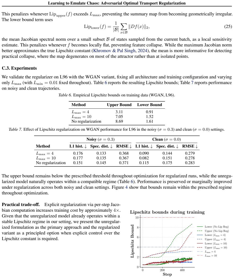
- Appendix C.1, Table 4: the WGAN row reports Jacobian spectral norms (min 1.290, max 2.126) that are consistently higher than Sinkhorn with early stopping (min 0.250, max 0.716). It would help to discuss whether this difference in Lipschitz regime affects the comparison between the two formulations.
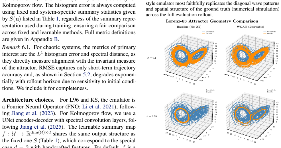
- Proposition A.1: the equality condition requires the Brenier map T* to be separable in the eigenbasis of C_T. The paper notes this 'provides some intuition' but the L63 visualizations in Figure 5 are used to support the practical relevance. It would be worth stating more explicitly how often this separability condition is expected to hold in practice.
- The paper uses 'Wasserstein noise forgetting' (Theorem 5.14) as a key term. This is evocative but could be confused with the standard notion of 'forgetting' in sequential learning. Consider clarifying that this refers to the decay of the initial-condition perturbation in the Wasserstein distance under the emulator's dynamics.
- References: the Peyré (2025) reference is to an arXiv preprint on 'Optimal transport for machine learners'; this appears to be a survey/lecture note and should be cited as such.
Simulated Author's Rebuttal
We thank the referee for a careful and constructive report. All three major comments identify genuine gaps that we will address in revision. On Comment 1 (exponential mixing assumption), we agree the connection between Theorem 5.14 and the experiments is weaker than presented and will add both an empirical mixing-rate diagnostic and a careful discussion of what LLE does and does not certify. On Comment 2 (Sinkhorn early stopping), we agree this is a significant practical limitation that deserves prominent discussion in the main text, and we will promote it from the appendix and clarify that WGAN is the more robust recommendation. On Comment 3 (mixed results), we agree the word 'consistently' overstates the findings and will revise the discussion to address the mixed and system-dependent patterns honestly.
read point-by-point responses
-
Referee: Theorem 5.14 assumes the emulator g is exponentially mixing in W_p (Definition 5.12), but the paper does not prove the trained emulator satisfies this property, nor does it directly verify it empirically. LLE matching is necessary but not sufficient for exponential mixing. The referee requests either (a) direct empirical verification of exponential mixing or (b) more careful discussion of what LLE does and does not show, with explicit acknowledgment that the theorem's applicability remains unverified.
Authors: The referee is correct on both counts. LLE measures local exponential divergence along a single trajectory and is indeed necessary but not sufficient for exponential mixing in W_p: a model could have the correct local expansion rate but wrong global recurrence structure. We will address this in two ways. First, we will add an empirical mixing-rate diagnostic: for each trained emulator, we estimate W_p((g∘k)_#η, ν) as k increases for several initial measures η (e.g., point masses, uniform on a grid, and the noisy observed measure), where ν is the empirical invariant measure estimated from a long emulator rollout. If the emulator is exponentially mixing, this quantity should decay geometrically; we will report the estimated rate ρ and compare it across methods. Second, we will revise the discussion around Table 3 to explicitly state that LLE matching provides evidence of correct local chaotic behavior but does not certify the global mixing property required by Theorem 5.14, and that the theorem's applicability to the trained models remains an assumption verified only empirically (not proven). The current presentation overstates the connection between the theorem and the experiments, and we will correct this. revision: yes
-
Referee: The Sinkhorn variant requires early stopping at 350/400 out of 500 training steps (Appendix C.1, Table 4) to avoid degenerate collapse of the summary map. Without early stopping, Jacobian spectral norms collapse near zero with rare large spikes, indicating the adversarial game does not converge to a meaningful equilibrium. This is a significant practical concern that should be discussed more prominently, not only in the appendix. The paper should clarify whether WGAN is the more robust recommendation and report sensitivity to the early stopping step.
Authors: We agree that this is a significant practical limitation that deserves prominent discussion in the main text, not only in the appendix. The Jacobian spectral norm statistics in Table 4 clearly show that the Sinkhorn min-max game can degenerate without early stopping, and this does suggest potential non-existence of a stable saddle point for the Sinkhorn formulation in our setting. We will make three changes: (1) promote the early-stopping discussion and Table 4 (or a summary thereof) from Appendix C.1 to the main text, likely in Section 6 or 7; (2) explicitly state that the WGAN variant, which does not require early stopping in any of our experiments, is the more robust practical recommendation; and (3) report sensitivity to the early stopping step by including results at multiple stopping points (e.g., 300, 350, 400, 450, 500) for at least one system. We will also note that the Sinkhorn instability is consistent with known challenges in adversarial training of learnable-cost OT objectives, and that the joint hinge regularization proposed in Appendix C.2 offers a principled (if more expensive) alternative for stabilizing the summary map. revision: yes
-
Referee: Table 2 shows mixed results: for L96 single-trajectory, Sinkhorn is better on clean but worse on noisy for L1 hist., and the reverse pattern appears for spectral distance. On KS single-trajectory noisy, Sinkhorn (L1 hist. 0.435) barely outperforms No OT (0.454). The paper should discuss these mixed results explicitly rather than stating that learnable OT methods 'consistently outperform' baselines.
Authors: The referee is correct that the results are more mixed than our current language suggests. The specific examples cited are accurate: on L96 single-trajectory, Sinkhorn and WGAN trade off between noisy and clean settings and between L1 histogram error and spectral distance; on KS noisy, Sinkhorn's L1 hist. error (0.435) is only marginally better than No OT (0.454), while WGAN achieves 0.339. The word 'consistently' overstates the pattern. We will revise the discussion in Section 7 to present a more nuanced and honest assessment: (1) both learnable OT methods substantially outperform No OT on spectral distance across all systems and conditions, which is the clearest and most consistent advantage; (2) on L1 histogram error, the advantage is system- and condition-dependent, with WGAN generally stronger on noisy data and Sinkhorn sometimes stronger on clean data; (3) on KS noisy, Sinkhorn's advantage over No OT on L1 hist. is marginal, and we will state this directly. We will also discuss the possibility that the Sinkhorn formulation's instability (Comment 2) contributes to its weaker noisy-data performance relative to WGAN. The revised text will replace 'consistently outperform' with a system-by-system and metric-by-metric summary. revision: yes
Circularity Check
No significant circularity: theoretical results are parameter-free derivations from stated assumptions; evaluation uses independent fixed metrics.
full rationale
The paper's theoretical results (Proposition 5.1, Theorem 5.14, Corollary 5.9) are standard mathematical derivations from explicitly stated assumptions (Lipschitz summary maps, exponential mixing, Gaussian noise). None of these assumptions embed the target conclusion as a hidden input. The key bound in Proposition 5.1 (W_{d_S^p}(f#µ, f#µ̂) ≤ L_f^p E[d_U(Φ(u), g(u))^p]) follows from constructing a feasible coupling and applying the Lipschitz property—a direct, non-circular derivation. Theorem 5.14's noise-forgetting result follows from the triangle inequality plus the exponential mixing assumption (Definition 5.12); while that assumption is strong and unverified for the learned emulator (a correctness concern, not a circularity concern), it does not encode the theorem's conclusion. The evaluation metrics (L1 histogram error, spectral distance) use fixed handcrafted summary statistics (Table 1) that are independent of the learned summaries, explicitly stated: 'The histogram error is always computed using fixed and system-specific summary statistics given by S(u) listed in Table 1, regardless of the summary representation used during training, ensuring a fair comparison.' The paper builds on Jiang et al. (2023) for architecture and data generation, but these are external citations to different authors. The one self-citation to Jiang et al. (2025) is for the UNet architecture used in the Kolmogorov flow experiments, which is not load-bearing for the theoretical claims. No step in the derivation chain reduces to its inputs by construction. The score of 1 reflects the minor, non-load-bearing nature of the architectural self-citation and the absence of any circular reasoning in the theoretical or experimental methodology.
Axiom & Free-Parameter Ledger
free parameters (5)
- λ (OT regularization weight) =
3 (L96), grid-searched (KS)
- ε (Sinkhorn entropic regularization) =
0.02 (L96, KS), 0.05 (L63)
- p (Wasserstein order) =
2 (Sinkhorn), 1 (WGAN)
- d (summary dimension) =
3 (default), 1 (ablation)
- Early stopping step (Sinkhorn) =
350/400 of 500
axioms (5)
- domain assumption The true dynamics Φ admits an invariant and ergodic probability measure μ on a compact attractor U.
- domain assumption The summary map f is L_f-Lipschitz.
- ad hoc to paper The emulator g is exponentially mixing in Wp with rate ρ∈(0,1).
- domain assumption Noise is additive isotropic Gaussian, independent of state.
- domain assumption The summary hypothesis class F contains a scaling map f(u)=L_f u when U⊆S⊆R^n.
invented entities (1)
-
Adversarial summary map f: U → S
independent evidence
Forward citations
Cited by 1 Pith paper
-
Data-Adaptive Learning of Dynamical Systems by Matching Transfer Operators and Invariant Measures
A data-adaptive operator-matching approach learns vector fields by aligning induced transition matrices and invariant measures on an unstructured partition, outperforming pointwise losses under noise.
Reference graph
Works this paper leans on
-
[1]
doi: 10.1017/jfm.2013.122. Chattopadhyay, A., Sun, Y . Q., and Hassanzadeh, P. Chal- lenges of learning multi-scale dynamics with ai weather models: Implications for stability and one solution, 2024. URLhttps://arxiv.org/abs/2304.07029. Cheng, X., He, Y ., Yang, Y ., Xue, X., Cheng, S., Giles, D., Tang, X., and Hu, Y . Learning chaos in a linear way. InPr...
-
[2]
doi: 10.1093/acprof: oso/9780198722588.001.0001
ISBN 9780198722588. doi: 10.1093/acprof: oso/9780198722588.001.0001. Dorfman, J. R.An Introduction to Chaos in Nonequilib- rium Statistical Mechanics. Cambridge Lecture Notes in Physics. Cambridge University Press, 1999. doi: 10.1017/CBO9780511628870. Feydy, J., S ´ejourn´e, T., Vialard, F.-X., ichi Amari, S., Trouv´e, A., and Peyr ´e, G. Interpolating be...
-
[3]
doi: https://doi.org/10.1016/ 0167-2789(86)90166-1
ISSN 0167-2789. doi: https://doi.org/10.1016/ 0167-2789(86)90166-1. Jakhar, K., Guan, Y ., Mojgani, R., Chattopadhyay, A., and Hassanzadeh, P. Learning closed-form equations for subgrid-scale closures from high-fidelity data: Promises and challenges.Journal of Advances in Modeling Earth Systems, 16(7):e2023MS003874, 2024. Jiang, R., Lu, P. Y ., Orlova, E....
work page 2024
-
[4]
How Well Do WGANs Estimate the Wasserstein Metric?
URL https://openreview.net/forum? id=c8P9NQVtmnO. Li, Z., Liu-Schiaffini, M., Kovachki, N., Azizzadenesheli, K., Liu, B., Bhattacharya, K., Stuart, A., and Anandku- mar, A. Learning chaotic dynamics in dissipative systems. InAdvances in Neural Information Processing Systems, volume 35, pp. 16768–16781, 2022. Lu, L., Jin, P., Pang, G., Zhang, Z., and Karni...
work page internal anchor Pith review Pith/arXiv arXiv doi:10.1038/s42256-021-00302-5 2022
-
[5]
Our learned MLP summary map is: ut 7→MLP(u t 1, ut 2)∈R 2×d
(∂tut 2,adv t 2, u t 2) ∈R 2×3. Our learned MLP summary map is: ut 7→MLP(u t 1, ut 2)∈R 2×d. In both cases, across the full trajectory you collectT×2vectors inR d as a point cloud. Overview of OT regularization strategies.We compare the fixed-statistics OT baseline introduced by Jiang et al. (2023) against two learnable OT-based regularizers. All three ap...
work page 2023
discussion (0)
Sign in with ORCID, Apple, or X to comment. Anyone can read and Pith papers without signing in.