Goodness of Fit Tests Based on Joint Densities of Multiple Sample Statistics
Pith reviewed 2026-07-03 07:33 UTC · model grok-4.3
The pith
Goodness-of-fit tests built from joint distributions of multiple sample statistics are competitive with and often more powerful than existing methods.
A machine-rendered reading of the paper's core claim, the machinery that carries it, and where it could break.
Core claim
The central claim is that goodness-of-fit tests can be constructed from simulated confidence sets for the joint distributions of multiple sample statistics, including order statistics, empirical distribution function values, moments, and combinations of classical statistics. One class uses hyperrectangular sets for principal-component vectors; the second uses highest density regions detected via k-nearest neighbors. These procedures are competitive with and often more powerful than existing methods in simulations, with extensions to two-sample permutation tests and transformations to target distributions such as the standard normal.
What carries the argument
Simulated confidence sets for the joint distribution of multiple sample statistics, which capture dependencies to define rejection regions for testing fit to a known continuous distribution.
If this is right
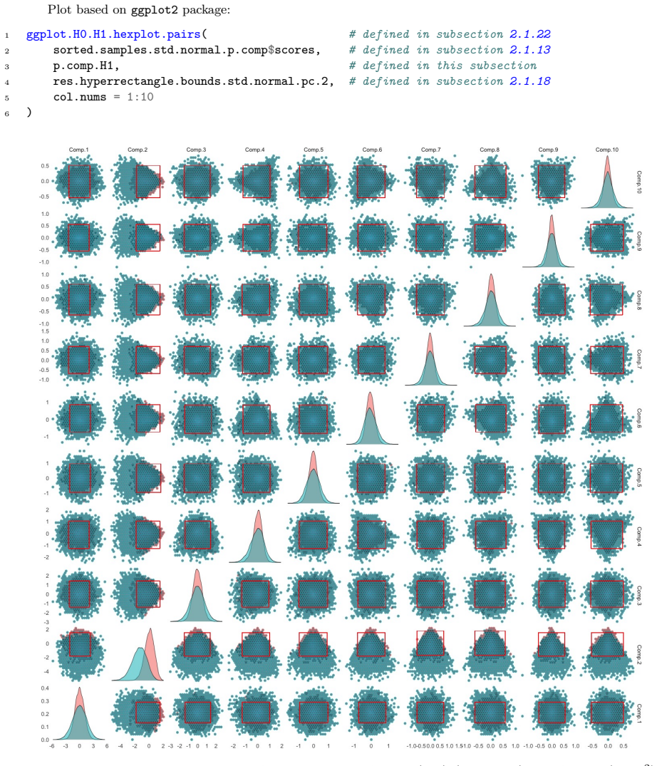
- Under a normal null the first principal component of the order statistics corresponds to the sample mean while the second relates to a linear analogue of variance.
- The methods extend to two-sample testing through permutation procedures based on the joint distributions of several statistics.
- Mapping data to another target distribution such as the standard normal can be advantageous when powerful tests exist for that distribution.
- Tests can be formed from combinations of classical goodness-of-fit statistics inside the highest-density-region framework.
Where Pith is reading between the lines
- The k-nearest-neighbor approach to highest density regions may extend more readily to higher-dimensional statistic vectors than kernel-density methods.
- The observed correspondence between principal components and mean-variance analogues under normality suggests that analogous geometric interpretations could be derived for other null distributions.
- If the joint-distribution approach generalizes, it could be applied to settings with estimated parameters by adjusting the simulation step accordingly.
Load-bearing premise
The null distributions are absolutely continuous with known parameters, which allows direct simulation of the joint distributions of the chosen sample statistics.
What would settle it
A simulation study against the alternatives examined in the paper in which the new tests show consistently lower power than Zhang or classical methods would falsify the claim of competitiveness and superior performance.
Figures


read the original abstract
We propose goodness-of-fit tests based on simulated confidence sets for joint distributions of multiple sample statistics, focusing on absolutely continuous null distributions with known parameters. One class of tests uses hyperrectangular confidence sets for principal components of order statistics and related statistic vectors. Extending earlier work on horizontal and vertical confidence bands for cumulative distribution functions, these tests are compared with some classical, Zhang, and related graphical tests. Simulations show that the proposed procedures are competitive with, and often more powerful than, existing methods. We also study the geometry of principal-component-based statistics; under a normal null distribution, the first principal component corresponds to the sample mean, while the second is related to a linear analogue of variance. A second class of tests uses confidence sets of arbitrary shape constructed through highest density regions. Unlike earlier kernel-density-based approaches, we use a k-nearest-neighbor method for detecting highest density regions, which is better suited to higher-dimensional statistic vectors. We study tests based on order statistics, empirical distribution function values, moments, and combinations of classical goodness-of-fit statistics. The resulting procedures are powerful against a wide range of alternatives. We also outline a two-sample extension via permutation tests based on joint distributions of several statistics and compare moment-based versions with energy-distance permutation tests. Finally, we discuss transformations other than the probability integral transform, showing that mapping data to another target distribution, such as the standard normal, can be advantageous when powerful tests are available for that distribution.
Editorial analysis
A structured set of objections, weighed in public.
Referee Report
Summary. The manuscript proposes goodness-of-fit tests for absolutely continuous null distributions with known parameters that rely on simulated confidence sets for the joint distribution of multiple sample statistics (order statistics, EDF values, moments, and classical GOF statistics). One class constructs hyperrectangular sets from principal components of these vectors; a second uses k-nearest-neighbor highest-density regions. The paper includes geometric analysis under normality (PC1 corresponds to the mean, PC2 to a linear variance analogue), power comparisons via simulation against classical, Zhang, and graphical tests, a permutation-based two-sample extension, and discussion of non-PIT transformations.
Significance. If the simulation results hold, the framework offers a flexible way to combine information across multiple statistics via joint density estimation, potentially yielding higher power against diverse alternatives than single-statistic or graphical methods. Explicit scoping to known-parameter continuous nulls enables direct Monte Carlo simulation of the joint distributions, which is a methodological strength. The k-NN approach for high-dimensional HDRs and the permutation two-sample procedure are practical extensions. The geometric interpretation under normality provides insight into what the PC-based tests are actually detecting.
major comments (1)
- The central empirical claim (Abstract) that the proposed procedures are 'competitive with, and often more powerful than, existing methods' rests entirely on simulations whose design (sample sizes, alternatives, number of Monte Carlo replications, handling of multiple statistics, and exact power metrics) is not summarized. Without these details it is impossible to assess whether the reported advantages are robust or sensitive to post-hoc selection of statistics or alternatives.
minor comments (3)
- The abstract mentions 'combinations of classical goodness-of-fit statistics' but does not list which classical statistics are included; a brief enumeration would clarify the scope of the second class of tests.
- The geometry discussion for the normal case (first PC = sample mean, second related to linear variance analogue) is stated without reference to the precise definition of the statistic vector or the PCA implementation; adding the relevant equation or definition would make the claim self-contained.
- The two-sample permutation extension is outlined only briefly; a short statement of how the joint distribution is estimated under the permutation null would improve readability.
Simulated Author's Rebuttal
We thank the referee for the positive assessment of the manuscript's contributions and for the recommendation of minor revision. We address the single major comment below.
read point-by-point responses
-
Referee: The central empirical claim (Abstract) that the proposed procedures are 'competitive with, and often more powerful than, existing methods' rests entirely on simulations whose design (sample sizes, alternatives, number of Monte Carlo replications, handling of multiple statistics, and exact power metrics) is not summarized. Without these details it is impossible to assess whether the reported advantages are robust or sensitive to post-hoc selection of statistics or alternatives.
Authors: We agree that the abstract would benefit from a concise summary of the simulation design to allow readers to evaluate the scope and robustness of the empirical results. In the revised manuscript we will expand the abstract to include the following details: sample sizes n=10,20,50,100; alternatives consisting of location, scale, and shape shifts under normal nulls together with t, chi-squared, uniform, and beta distributions; 10,000 Monte Carlo replications for power estimation (with 5,000 used for critical-value calibration); and handling of multiple statistics via pre-specified fixed combinations (order statistics, EDF ordinates, moments, and classical GOF statistics) chosen on the basis of the geometric analysis in Section 3 rather than data-driven selection. The power metric is the empirical rejection rate at nominal level 0.05. These additions will make the design transparent while preserving the abstract's brevity; the full experimental protocol remains in Section 4. revision: yes
Circularity Check
No significant circularity
full rationale
The paper proposes Monte Carlo-based goodness-of-fit procedures that simulate joint distributions of chosen statistics (order statistics, EDF values, moments) directly from the known absolutely continuous null. Power claims rest on external simulation comparisons to named existing tests rather than any internal derivation that reduces performance metrics to quantities defined by the method itself. No equations equate a 'prediction' to a fitted input, no self-citation chain supplies a uniqueness theorem or ansatz, and the geometry remarks follow from standard PCA properties. The derivation chain is therefore self-contained against external benchmarks.
Axiom & Free-Parameter Ledger
free parameters (2)
- choice and number of sample statistics
- k for nearest-neighbor density estimation
axioms (1)
- domain assumption Null distribution is absolutely continuous with known parameters
Reference graph
Works this paper leans on
-
[1]
Adler and Jonathan E
Robert J. Adler and Jonathan E. Taylor. Random Fields and Geometry . Springer, 2007
2007
-
[2]
Monte Carlo implementation of a guiding-center Fokker-Planck kinetic equation
Sivan Aldor-Noiman, Lawrence D. Brown, Andreas Buja, Wolfgang Rolke, and Robert A. Stine. The power to see: A new graphical test of normality. The American Statistician , 67(4):249–260, 2013. doi: 10.1080/00031305.2013.847865
work page internal anchor Pith review Pith/arXiv arXiv doi:10.1080/00031305.2013.847865 2013
-
[3]
T. W. Anderson and D. A. Darling. Asymptotic theory of certain ”goodness-of-fit” criteria based on stochastic processes. Annals of Mathematical Statistics , 23(2):193–212, 1952. doi:10.1214/aoms/ 1177729437
-
[4]
T. W. Anderson and D. A. Darling. A test of goodness of fit. Journal of the American Statistical Association, 49(268):765–769, 1954. doi:10.1080/01621459.1954.10501232
-
[5]
Testing density forecasts, with applications to risk management
Jeremy Berkowitz. Testing density forecasts, with applications to risk management. Journal of Business & Economic Statistics , 19(4):465–474, 2001. doi:10.1198/07350010152596718
-
[6]
FNN: Fast Nearest Neighbor Search Algorithms and Applications , 2024
Alina Beygelzimer, Sham Kakadet, John Langford, Sunil Arya, David Mount, and Shengqiao Li. FNN: Fast Nearest Neighbor Search Algorithms and Applications , 2024. R package version 1.1.4.1. URL: https: //CRAN.R-project.org/package=FNN
2024
-
[7]
Calibration for simultaneity: (re)sampling methods for simultaneous inference with applications to function estimation and functional data
Andreas Buja and Wolfgang Rolke. Calibration for simultaneity: (re)sampling methods for simultaneous inference with applications to function estimation and functional data. Working paper, 2006. URL: http://stat.wharton.upenn.edu/~buja/PAPERS/paper-sim.pdf
2006
-
[8]
hexbin: Hexagonal Binning Routines, 2024
Dan Carr, Nicholas Lewin-Koh, Martin Maechler, and Deepayan Sarkar. hexbin: Hexagonal Binning Routines, 2024. R package version 1.28.5. URL: https://CRAN.R-project.org/package=hexbin
2024
-
[9]
Christian T. Covington and Jeffrey W. Miller. A powerful goodness-of-fit test using the probability integral transform of order statistics, 2025. URL: https://arxiv.org/abs/2510.22854, arXiv:2510.22854
-
[10]
On the composition of elementary errors.Scandinavian Actuarial Journal, 1928(1):13–74,
Harald Cram´ er. On the composition of elementary errors.Scandinavian Actuarial Journal, 1928(1):13–74,
1928
-
[11]
doi:10.1080/03461238.1928.10416862
-
[12]
H. A. David and H. N. Nagaraja. Order Statistics. Wiley, 2003
2003
-
[13]
Karhunen-lo` eve expansions of mean-centered wiener processes.IMS Lecture Notes, 2006
Paul Deheuvels. Karhunen-lo` eve expansions of mean-centered wiener processes.IMS Lecture Notes, 2006
2006
-
[14]
Alternative approaches for estimating highest-density regions
Nina Deliu and Brunero Liseo. Alternative approaches for estimating highest-density regions. Inter- national Statistical Review , 94(1):97–120, 2026. URL: https://onlinelibrary.wiley.com/doi/abs/10. 1111/insr.12592, arXiv:2401.00245, doi:10.1111/insr.12592
-
[15]
Alain Desgagn´ e and Fr´ ed´ eric Ouimet. Omnibus goodness-of-fit tests for univariate continuous distri- butions based on trigonometric moments. Statistica Neerlandica, 80(2):e70025, 2026. URL: https:// onlinelibrary.wiley.com/doi/abs/10.1111/stan.70025, arXiv:https://onlinelibrary.wiley.com/ doi/pdf/10.1111/stan.70025, doi:10.1111/stan.70025
-
[16]
Rcpp: Seamless r and c++ integration
Dirk Eddelbuettel and Romain Francois. Rcpp: Seamless r and c++ integration. Journal of Statistical Software, 40(8):1–18, 2011. doi:10.18637/jss.v040.i08
-
[17]
Rcpp: Seamless R and C++ Integration , 2026
Dirk Eddelbuettel, Romain Francois, et al. Rcpp: Seamless R and C++ Integration , 2026. R package version 1.1.1. URL: https://CRAN.R-project.org/package=Rcpp
2026
-
[18]
Rob J. Hyndman. Computing and graphing highest density regions. The American Statistician, 50(2):120– 126, 1996. doi:10.1080/00031305.1996.10474359
work page internal anchor Pith review Pith/arXiv arXiv doi:10.1080/00031305.1996.10474359 1996
-
[19]
Programming languages — c++, 2020
International Organization for Standardization. Programming languages — c++, 2020
2020
-
[20]
¨Uber lineare methoden in der wahrscheinlichkeitsrechnung
Kari Karhunen. ¨Uber lineare methoden in der wahrscheinlichkeitsrechnung. 1947. In German
1947
-
[21]
King, Xibin Zhang, and Muhammad Akram
Maxwell L. King, Xibin Zhang, and Muhammad Akram. Hypothesis testing based on a vector of statis- tics. Journal of Econometrics , 219(2):425–455, 2020. Annals Issue: Econometric Estimation and Test- ing: Essays in Honour of Maxwell King. URL: https://www.sciencedirect.com/science/article/pii/ S0304407620301056, doi:10.1016/j.jeconom.2020.03.010. 164
-
[22]
A. N. Kolmogorov. On the empirical determination of a distribution law. Giornale dell’Istituto Italiano degli Attuari, 4:83–91, 1933. Originally published in Italian as ”Sulla determinazione empirica di una legge di distribuzione”
1933
-
[23]
Fonctions al´ eatoires de second ordre
Michel Lo` eve. Fonctions al´ eatoires de second ordre. 1948. In French
1948
-
[24]
Springer, 1977
Michel Lo` eve.Probability Theory I . Springer, 1977
1977
-
[25]
Marhuenda, D
Y. Marhuenda, D. Morales, and M. C. Pardo. A comparison of uniformity tests. Statistics, 39(4):315–327,
-
[26]
doi:10.1080/02331880500178562
-
[27]
David Novoa-Paradela, Oscar Fontenla-Romero, and Bertha Guijarro-Berdi˜ nas. A one-class classification method based on expanded non-convex hulls. Information Fusion, 89:1–15, 2023. doi:10.1016/j.inffus. 2022.07.023
-
[28]
Chatgpt (gpt-5.5)
OpenAI. Chatgpt (gpt-5.5). https://chatgpt.com/, 2026. Large language model accessed May 15, 2026
2026
-
[29]
ggrastr: Rasterize Layers for ’ggplot2’ ,
Viktor Petukhov, Teun van den Brand, and Evan Biederstedt. ggrastr: Rasterize Layers for ’ggplot2’ ,
-
[30]
URL: https://CRAN.R-project.org/package=ggrastr
R package version 1.0.2. URL: https://CRAN.R-project.org/package=ggrastr
-
[31]
R: A Language and Environment for Statistical Computing
R Core Team. R: A Language and Environment for Statistical Computing . R Foundation for Statistical Computing, Vienna, Austria, 2026. URL: https://www.R-project.org/
2026
-
[32]
Ramsay and Bernard W
James O. Ramsay and Bernard W. Silverman. Functional Data Analysis . Springer, 2005
2005
-
[33]
Supplemental studies for simultaneous goodness-of-fit testing, 2020
Wolfgang Rolke. Supplemental studies for simultaneous goodness-of-fit testing, 2020. URL: https:// arxiv.org/abs/2007.04727, arXiv:2007.04727
-
[34]
Simulation studies for goodness-of-fit and two-sample methods for univariate data
Wolfgang Rolke. Simulation studies for goodness-of-fit and two-sample methods for univariate data. arXiv preprint arXiv:2411.05839, November 2024. URL: https://arxiv.org/abs/2411.05839
-
[35]
Rom˜ ao, R
X. Rom˜ ao, R. Delgado, and A. Costa. An empirical power comparison of univariate goodness-of-fit tests for normality. Journal of Statistical Computation and Simulation , 80(5):545–591, 2010. doi:10.1080/ 00949650902740824
2010
-
[36]
Teemu S¨ ailynoja, Paul-Christian B¨ urkner, and Aki Vehtari. Graphical test for discrete uniformity and its applications in goodness-of-fit evaluation and multiple sample comparison. Statistics and Computing , 32(2):1–21, 2022. doi:10.1007/s11222-022-10090-6
-
[37]
Lattice: Multivariate Data Visualization with R
Deepayan Sarkar. Lattice: Multivariate Data Visualization with R . Springer, New York, 2008. URL: http://lmdvr.r-forge.r-project.org
2008
-
[38]
GGally: Extension to ’ggplot2’ , 2024
Barret Schloerke, Di Cook, Joseph Larmarange, Francois Briatte, Moritz Marbach, Edwin Thoen, Amos Elberg, and Jason Crowley. GGally: Extension to ’ggplot2’ , 2024. R package version 2.2.1. URL: https: //CRAN.R-project.org/package=GGally
2024
-
[39]
Shorack and Jon A
Galen R. Shorack and Jon A. Wellner. Empirical Processes with Applications to Statistics . SIAM, 1986
1986
-
[40]
Shorack and Jon A
Galen R. Shorack and Jon A. Wellner. Empirical Processes with Applications to Statistics . Wiley Series in Probability and Mathematical Statistics. Wiley, New York, 1986
1986
-
[41]
Yilun Du, Shuang Li, Antonio Torralba, Joshua B
Michael A. Stephens. Edf statistics for goodness of fit and some comparisons. Journal of the American Statistical Association, 69(347):730–737, 1974. doi:10.1080/01621459.1974.10480196
-
[42]
W. N. Venables and B. D. Ripley. Modern Applied Statistics with S . Springer, New York, fourth edition,
-
[43]
URL: https://www.stats.ox.ac.uk/pub/MASS4/
ISBN 0-387-95457-0. URL: https://www.stats.ox.ac.uk/pub/MASS4/
-
[44]
Wahrscheinlichkeitsrechnung und ihre Anwendung auf die Statistik und theoretische Physik
Richard von Mises. Wahrscheinlichkeitsrechnung und ihre Anwendung auf die Statistik und theoretische Physik. F. Deuticke, Leipzig, 1931. In German; English translation published as Probability, Statistics and Truth (1939, Macmillan)
1931
-
[45]
Probability, Statistics and Truth
Richard von Mises. Probability, Statistics and Truth . Macmillan, New York, 1939. English translation of Wahrscheinlichkeitsrechnung und ihre Anwendung auf die Statistik und theoretische Physik (1931)
1939
-
[46]
Application of equal local levels to improve q-q plot testing bands with r package qqconf
Eric Weine, Mary Sara McPeek, and Mark Abney. Application of equal local levels to improve q-q plot testing bands with r package qqconf. Journal of Statistical Software , 106(10):1–33, 2023. URL: https://www.jstatsoft.org/article/view/v106i10, doi:10.18637/jss.v106.i10
-
[47]
ggplot2: Elegant Graphics for Data Analysis
Hadley Wickham. ggplot2: Elegant Graphics for Data Analysis . Springer-Verlag New York, 2016. URL: https://ggplot2.tidyverse.org
2016
-
[48]
Powerful Goodness-of-Fit Tests and Multi-Sample Tests
Jin Zhang. Powerful Goodness-of-Fit Tests and Multi-Sample Tests . PhD thesis, York University, Toronto, Canada, 2001
2001
-
[49]
Powerful goodness-of-fit tests based on the likelihood ratio
Jin Zhang. Powerful goodness-of-fit tests based on the likelihood ratio. Journal of the Royal Statistical Society: Series B (Statistical Methodology) , 64(2):281–294, 2002. doi:10.1111/1467-9868.00337. 165
discussion (0)
Sign in with ORCID, Apple, or X to comment. Anyone can read and Pith papers without signing in.